Time and Space Complexity Analysis

Asymptotic notation says how to compare growth rates. This note shows how to obtain the function to compare: how to count the work done by loops, nested loops and recursive calls, and how much memory a program needs beyond its input. The counts below reduce to one of the loop patterns, an exact iteration count, or a stack-depth argument.

Analysis assumes the RAM model (CLRS 3e, Section 2.2): instructions run one after another, and each basic operation (arithmetic on word-sized numbers, comparison, assignment, array indexing, a function call and return) takes constant time. Running time is then proportional to the number of basic operations executed.

Two choices must be stated for every analysis:

The input-size choice matters. Trial division tests whether $N$ is prime with about $\sqrt{N}$ divisions. That is polynomial in the value $N$ but $2^{b/2}$ in the number of bits $b$, so it is exponential in the input size. Algorithms polynomial in the numeric value but not in its bit length are called pseudo-polynomial; the $O(nW)$ 0/1 knapsack algorithm is the standard example.

A geometric series is dominated by its largest term: an increasing one is $\Theta(\text{last term})$ and a decreasing one is $\Theta(\text{first term})$.

Pseudocode is CLRS-like: <- is assignment, loops are inclusive of both bounds, and arrays are 1-indexed.

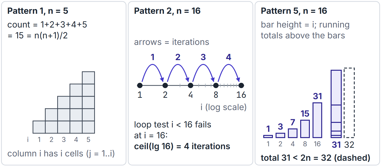
The inner loop runs $i$ times, so $\text{count} = \sum_{i=1}^{n} i = n(n+1)/2 = \Theta(n^2)$. Halving the work (a triangle instead of a square) does not change the order. With three nested loops $1 \le i < j < k \le n$ the count is $\binom{n}{3} = \Theta(n^3)$.

After $t$ iterations $i = 2^t$, and the loop stops when $2^t \ge n$. So it runs exactly $\lceil \lg n \rceil$ times for $n \ge 1$ (for example 7 times for $n = 100$, 10 for $n = 1024$, 11 for $n = 1025$). Halving loops (i <- floor(i/2) until $i = 0$) behave the same way: $\lfloor \lg n \rfloor + 1$ iterations from $i = n \ge 1$. The base of the multiplication only changes the constant: multiplying by 3 gives $\lceil \log_3 n \rceil = \Theta(\lg n)$.

The inner loop runs $\lfloor \lg i \rfloor + 1$ times, so the total is $\sum_{i=1}^{n} (\lfloor \lg i \rfloor + 1) = \Theta(\lg(n!)) = \Theta(n \lg n)$. For $n = 8$ the counts are 1, 2, 2, 3, 3, 3, 3, 4, total 21.

For a fixed $i$ the inner loop runs $\lceil n/i \rceil$ times. The total is $\sum_{i=1}^{n} \lceil n/i \rceil$, which lies between $n H_n$ and $n H_n + n$, so it is $\Theta(n \lg n)$. For $n = 10$: $10 + 5 + 4 + 3 + 2 + 2 + 2 + 2 + 2 + 1 = 33$. This pattern appears in the sieve of Eratosthenes and in "for each divisor" loops.

The inner loop runs $1, 2, 4, \ldots, 2^k$ times, where $2^k \le n < 2^{k+1}$. The total $2^{k+1} - 1$ is less than $2n$, so the fragment is $\Theta(n)$, not $\Theta(n \lg n)$. For $n = 16$ the total is 31. Multiplying the number of outer iterations ($\lg n$) by the largest inner count ($n$) gives only an upper bound.

If $n = 2^{2^k}$, the values are $2^{2^k}, 2^{2^{k-1}}, \ldots, 2^{2} = 4, 2$, so the loop runs $k = \lg \lg n$ times: 4 times for $n = 65536$. In general the count is $\Theta(\lg \lg n)$.

The inner while can run up to $n$ times for one $i$, but $j$ never decreases and never exceeds $n + 1$, so the inner body runs at most $n$ times in total. The fragment is $\Theta(n)$ in the worst case, not $\Theta(n^2)$. Always ask whether an inner index is reset; this is the key to merge, two-pointer scans and BFS-style analyses.

The left loop runs $\lfloor \sqrt{n} \rfloor$ times (10 for $n = 100$, 9 for $n = 99$). In the right loop, after $t$ iterations $s = t(t+1)/2$, so it stops at the least $t$ with $t(t+1)/2 \ge n$: $t = \Theta(\sqrt{n})$, 14 for $n = 100$ (since $13 \cdot 14/2 = 91 < 100 \le 105$). A loop variable that grows by an increasing step is the usual disguise of $\Theta(\sqrt{n})$.

The outer loop takes $i = 2^t$ for $t = 0, 1, \ldots, T - 1$ with $T = \lceil \lg n \rceil$, and the inner loop runs $t$ times for $i = 2^t$. The total is $0 + 1 + \cdots + (T-1) = T(T-1)/2 = \Theta(\lg^2 n)$: 45 for $n = 1024$ ($T = 10$), 55 for $n = 1025$ ($T = 11$). Neither $\Theta(\lg n)$ nor $\Theta(n)$ is right.

The count is the number of triples $1 \le k \le j \le i \le n$, which is $\binom{n+2}{3} = n(n+1)(n+2)/6$: 20 for $n = 4$, 220 for $n = 10$. With strict inequalities ($k < j < i$) it is $\binom{n}{3}$ instead. Both are $\Theta(n^3)$, but an exact-count question distinguishes them.

Linear search for a key $x$ in $A[1..n]$:

The average case needs an explicit assumption; here, that $x$ is present and equally likely at each position. Change the assumption (for example, $x$ absent with probability $1/2$) and the exact average changes, though here it stays $\Theta(n)$.

"Space complexity" may mean auxiliary space or total space; check the wording. An algorithm is in place if it uses $O(1)$ auxiliary space apart from the input. Some books also call quicksort in place although its stack uses $O(\lg n)$ to $O(n)$ words; when it matters, state which convention is meant.

Each active call keeps a stack frame (parameters, locals, return address) of constant size in typical analyses. Auxiliary space for recursion is therefore $\Theta(\text{maximum recursion depth})$ times the frame size, not the total number of calls.

Here $\phi=(1+\sqrt{5})/2$ is the golden ratio.

The Fibonacci row shows the distinction clearly: exponential time, linear space, because only one root-to-leaf path of calls is on the stack at any moment. (Call counts are taken with base cases $F(0)$ and $F(1)$; see Recursion Tracing and Call Counting.)

Memory can buy time. Storing the Fibonacci values computed so far (dynamic programming) cuts time from exponential to $\Theta(n)$ at the cost of $\Theta(n)$ space, or $\Theta(1)$ space if only the last two values are kept. A hash table trades $\Theta(n)$ space for expected $O(1)$ lookups.