
Introduction
Dynamic programming (DP) solves an optimisation (or counting) problem by combining answers to smaller overlapping subproblems. Where plain recursion recomputes the same subproblem many times, DP stores each answer once and reuses it. Where a greedy algorithm commits to one local choice, DP considers every feasible choice at a subproblem and keeps the best.
The GATE syllabus names DP as a design technique. This note states the two ingredients (optimal substructure and overlapping subproblems), shows the memoized and bottom-up styles on the classical rod-cutting problem, and records how to reconstruct a solution from a filled table. Concrete applications (LCS, knapsack, matrix-chain, Floyd-Warshall) live in later notes.
Prerequisites
- Solving Recurrences and the Master Theorem: reading the cost of a recursive formulation.
- Recursion: call trees and memoization as caching of recursive calls.
Core concepts
Two ingredients
- Optimal substructure. An optimal solution of the instance contains optimal solutions of smaller instances. Formally: if you cut an optimal rod solution after the first piece of length , the remaining length is itself cut optimally.
- Overlapping subproblems. The natural recursion revisits the same smaller instance many times. In many polynomial-time examples here the number of distinct states is polynomial while the recursion tree has exponential size. Overlap means repeated states; DP time is determined by the actual state and transition counts, which need not be polynomial.
Divide and conquer also needs optimal (or exact) substructure, but its subproblems are independent: merge sort never sorts the same index range twice. Memoizing merge sort therefore gains nothing. DP is the right tool precisely when the same subproblem recurs.
Two implementation styles
| Style | Idea | Typical time | Extra space |
|---|---|---|---|
| Top-down (memoization) | Recurse as usual; cache every return value in a table keyed by the subproblem | Same as bottom-up, up to recursion overhead | Table of all reached states, plus the call stack |
| Bottom-up (tabulation) | Enumerate subproblems from smallest to largest and fill a table in that order | The table (often compressible to a few rows) |
Both compute the same values. Bottom-up makes the fill order explicit and avoids stack overflow; top-down computes only states that are actually needed.
Fill order. A bottom-up table must be filled so that every state is computed after all the states it reads. If reads and (LCS, edit distance, knapsack), row-major order works. If it reads shorter intervals and (matrix-chain), fill by increasing interval length ; plain row-major order from the top row would read cells that are not yet filled.
State, transition, base case
A DP solution is completely described by:
- the state (what identifies a subproblem),
- the recurrence / transition (how a state's answer is built from smaller ones),
- the base cases,
- and, when a concrete solution is required, the reconstruction rule (often an auxiliary choice table).
Writing these four items before coding is the reliable habit.
Algorithms and pseudocode
Pseudocode uses 1-based arrays, <- for assignment and A[i..j] for the subarray from position to position .
Rod cutting
Input. A rod of integer length and a price list , where is the price of a piece of length .
Output. The maximum revenue obtainable by cutting the rod into integer-length pieces (or leaving it uncut). Cuts are free.
Optimal substructure gives the recurrence
Here is the length of the first piece; the residual rod of length is solved optimally. The case is the uncut rod.
MEMOIZED-CUT-ROD(p, n)
1  let r[0..n] be a new array
2  for i <- 0 to n
3      r[i] <- -infinity
4  return MEMOIZED-CUT-ROD-AUX(p, n, r)

MEMOIZED-CUT-ROD-AUX(p, n, r)
1  if r[n] != -infinity then
2      return r[n]
3  if n = 0 then
4      q <- 0
5  else q <- -infinity
6      for i <- 1 to n
7          q <- max(q, p[i] + MEMOIZED-CUT-ROD-AUX(p, n - i, r))
8  r[n] <- q
9 return qBOTTOM-UP-CUT-ROD(p, n)
1 let r[0..n] be a new array
2 r[0] <- 0
3 for j <- 1 to n
4 q <- -infinity
5 for i <- 1 to j
6 q <- max(q, p[i] + r[j - i])
7 r[j] <- q
8 return r[n]Time / space. Bottom-up: the outer loop runs times and the inner loop up to times, so time and space. Memoized: the same asymptotic bounds; each of the distinct lengths is solved once, and solving length costs . Naive recursion without a table is (CLRS 3e, Section 15.1).
Reconstruction. Store with each the first-piece length that attained the maximum. Then emit pieces by walking until length 0.
EXTENDED-BOTTOM-UP-CUT-ROD(p, n)
1  let r[0..n] and s[0..n] be new arrays
2  r[0] <- 0
3  for j <- 1 to n
4      q <- -infinity
5      for i <- 1 to j
6          if q < p[i] + r[j - i] then
7              q <- p[i] + r[j - i]
8              s[j] <- i
9      r[j] <- q
10 return (r, s)

PRINT-CUT-ROD-SOLUTION(p, n)
1  (r, s) <- EXTENDED-BOTTOM-UP-CUT-ROD(p, n)
2  while n > 0
3      print s[n]
4      n <- n - s[n]
Edge cases. returns revenue 0 and no pieces. The full rod length must be consumed, even with negative prices. For , , , the best cut is , with revenue , not the uncut piece. The memoized algorithm uses a reserved sentinel, distinct from all finite revenues; the examples here use positive prices. Ties among several optimal first pieces are broken by the if q < ... test (the smallest wins); any tie-break is correct for the revenue.
Mathematical explanation
Why the recurrence is correct
Let be any optimal cutting of a rod of length , and let the leftmost piece have length . The remaining pieces form a cutting of length . If that residual cutting were suboptimal, replacing it by an optimal one would raise the total revenue, contradicting optimality of . Hence some optimal solution begins with a first piece of length followed by an optimal solution of length . Maximising over every feasible yields .
Overlap count
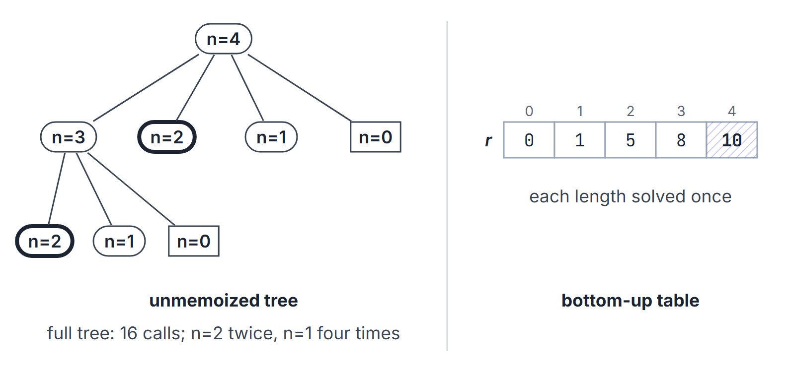
A naive recursive call for length spawns calls for every smaller length; those in turn spawn further calls. If counts all calls, and , so . The recursion tree has leaves for : each composition of as an ordered sum of positive integers is one root-to-leaf path. Distinct subproblems, however, are only the lengths . Memoization collapses the exponential tree onto a linear table.
Pseudo-polynomial time
Running time is measured against the input size in bits. A number occupies about bits, so a bound like (0/1 knapsack, coin change for amount ) is polynomial in the value but exponential in its length: doubling the number of bits of squares . Such an algorithm is called pseudo-polynomial. It is fast when the numbers are small, and it does not contradict the NP-hardness of 0/1 knapsack. By contrast, rod cutting's bound is polynomial in the input size, since the input lists prices.
DP versus greedy versus divide and conquer
| Optimal substructure | Overlapping subproblems | Choice at a state | |
|---|---|---|---|
| DP | required | required (else memoization is pointless) | try all, keep best |
| Greedy | required | not needed | commit to one local rule |
| Divide and conquer | required for correctness of the combine | absent (independent subproblems) | fixed split, then combine |
A density-greedy cut for rod cutting fails on the prices for : density picks length 3 first (revenue ), while two pieces of length 2 give (CLRS Exercise 15.1-2).
Worked examples
Rod cutting for
Prices (CLRS Figure 15.1 style): .
Bottom-up fill:
| candidates | |||
|---|---|---|---|
| 1 | 1 | 1 | |
| 2 | , | 5 | 2 |
| 3 | , , | 8 | 3 |
| 4 | , , , | 10 | 2 |
Revenue , first piece , residual length 2 with : pieces . The uncut rod is worth only 9.
Fibonacci as a counting DP
The recurrence , , for has optimal-substructure form (exactly two subproblems) and massive overlap. Bottom-up fills an array in time; with the golden ratio , the naive tree has nodes. This is a counting / evaluation DP rather than an optimisation DP, but the same two ingredients apply (CLRS Exercise 15.1-5).
Counting DP: ways to pay an amount
Count the ways to pay 5 with coins of value 1, 2 and 5 (unlimited supply).
- Combinations (order does not matter, ): process coins in the outer loop, for , after initializing , then . Result 4: .
- Ordered sequences ( and are different): independently reset all entries ways[0..5] to zero and set ways[0]=1; put amounts in the outer loop, . Result 9.
Loop order versus meaning. The same one-line recurrence counts different things depending on which loop is outside. Coins outside gives combinations (4); amounts outside gives ordered sequences (9).
The minimum number of coins uses the same shape with : , . For coins 1, 2 and 5 and amount 11 it gives 3 ().
Counting calls in naive recursion
Plain recursive Fibonacci (fib(n) calls fib(n-1) and fib(n-2), with fib(0) and fib(1) as base cases) makes calls in total. For that is 15 calls: fib(2) runs 3 times, fib(1) 5 times and fib(0) 3 times. With memoization each of fib(0) to fib(5) is computed once, in total time.
When not to use DP
- Independent subproblems (binary search, merge sort): divide and conquer.
- A proved greedy-choice property (activity selection, Huffman, MST): greedy is enough and usually faster.
- Simple-path constraints require care. With nonnegative weights, or when no relevant negative cycle exists, shortest-walk optimal substructure applies: subpaths of shortest paths are shortest. For arbitrary signed weights, shortest and longest simple paths may require visited-set states to enforce simplicity; those states can be exponential. A state consisting only of endpoints cannot in general encode the interaction between already visited vertices.
Important properties and observations
- The table size equals the number of distinct states. If a state needs two indices with , expect states (matrix-chain, LCS with two strings of length ).
- Time is (states) times (work to compute one state). Rod cutting: states, work each, total.
- Space can often drop to the last row or two when reconstruction is not required (LCS length alone needs space).
- Reconstruction needs either an explicit choice table or a second pass that re-evaluates the recurrence and follows the argmax.
- Always state whether the problem asks for the optimal value, one optimal solution, or the number of optimal solutions: the three variants share a table shape but differ in the transition and in what is stored.
Common misconceptions.
- "DP is recursion with a table." Memoization is that; bottom-up DP never needs a recursive call.
- "Greedy is a special case of DP." Greedy commits without comparing alternatives; DP compares them. They share optimal substructure, not the choice rule.
- "Every overlapping recursion is DP." If the goal is not built from sub-answers by a fixed combine (for example, searching for any feasible path with side constraints that break optimal substructure), caching alone does not yield a correct algorithm.
GATE examination perspective
- IDENTIFY THE STATE. Given a verbal problem, first fix the dimension of the DP table and the meaning of .
- WRITE THE RECURRENCE FIRST. Fill-order and complexity follow from the recurrence; coding without it invites off-by-one errors.
- COUNT THE STATES AND THE TRANSITIONS. Time .
- RECONSTRUCTION. Be ready to recover the cuts, the parenthesization or the subsequence from the choice table.
- GREEDY COUNTEREXAMPLE. A one-line instance where density (or another local rule) fails shows why DP is needed.
- CALL COUNTS. "How many times is
f(k)called?" Draw the first levels of the naive tree or set up a count recurrence; memoization reduces each count to one computation. - WAYS TO PAY. Coins in the outer loop count combinations; amounts in the outer loop count ordered sequences.
- PSEUDO-POLYNOMIAL. is not polynomial in the input size when is given in binary.
Summary
Sources
- T. H. Cormen, C. E. Leiserson, R. L. Rivest, C. Stein, Introduction to Algorithms, 3rd ed., MIT Press, 2009: Chapter 15, Section 15.1 (rod cutting) and Section 15.3 (elements of dynamic programming); Exercises 15.1-2 (greedy density counterexample) and 15.1-5 (Fibonacci).