
Introduction
Sorting rearranges records so that their keys are in non-decreasing order. Bubble sort, selection sort and insertion sort are the three simple quadratic methods. Their worst-case quadratic cost is slower than merge sort or heapsort on large inputs, but they are short and in place. Insertion sort is especially suitable for small or nearly sorted arrays and is used inside fast library sorts for small subarrays. They are also the clearest place to learn the properties every sorting question asks about: comparisons, swaps, stability, adaptivity and inversions.
Prerequisites
- Time and Space Complexity Analysis: counting nested loops, best and worst case.
- Arrays with 1-based indexing, as in the pseudocode below.
Core concepts
Properties used to classify sorts
- In place. uses auxiliary memory besides the input array.
- Stable. records with equal keys keep their original relative order. Stability matters when sorting by one key after another (sort by name, then stably by city, and names stay sorted within each city).
- Adaptive. runs faster on input that is already nearly sorted.
- Online. can sort the input as it arrives, one element at a time.
- Comparison-based. examines keys only by comparing pairs. All three sorts here are comparison-based, so the lower bound of Comparison of Sorting Algorithms applies to them.
Inversions
An inversion of is a pair of positions with and . The number of inversions measures how unsorted the array is:
- exactly when the array is sorted.
- , the maximum, exactly when the array is in strictly decreasing order.
- Averaged over all orderings of distinct keys, : each of the pairs is inverted in exactly half of the orderings.
- Swapping unequal adjacent keys changes by exactly 1; swapping equal keys leaves unchanged. So any sort that only exchanges adjacent elements (bubble sort, insertion sort) performs at least exchanges, and is on average.
Example: has inversions: , , , , , , , , .
Insertion sort
Idea. Keep a sorted prefix . Insert into it by shifting larger elements one place right. Input. . Output. sorted in place.
Pseudocode uses 1-based arrays, <- for assignment and A[i..j] for the subarray from position to position .
INSERTION-SORT(A, n)
    for j <- 2 to n
        key <- A[j]
        i <- j - 1
        while i > 0 and A[i] > key
            A[i + 1] <- A[i]
            i <- i - 1
        A[i + 1] <- key
Invariant. At the start of each iteration, holds the original first elements in sorted order.
Trace on :
| key | Array after inserting key | Shifts | |
|---|---|---|---|
| 2 | 2 | 2 5 4 6 1 3 | 1 |
| 3 | 4 | 2 4 5 6 1 3 | 1 |
| 4 | 6 | 2 4 5 6 1 3 | 0 |
| 5 | 1 | 1 2 4 5 6 3 | 4 |
| 6 | 3 | 1 2 3 4 5 6 | 3 |
Total shifts ; total key comparisons .
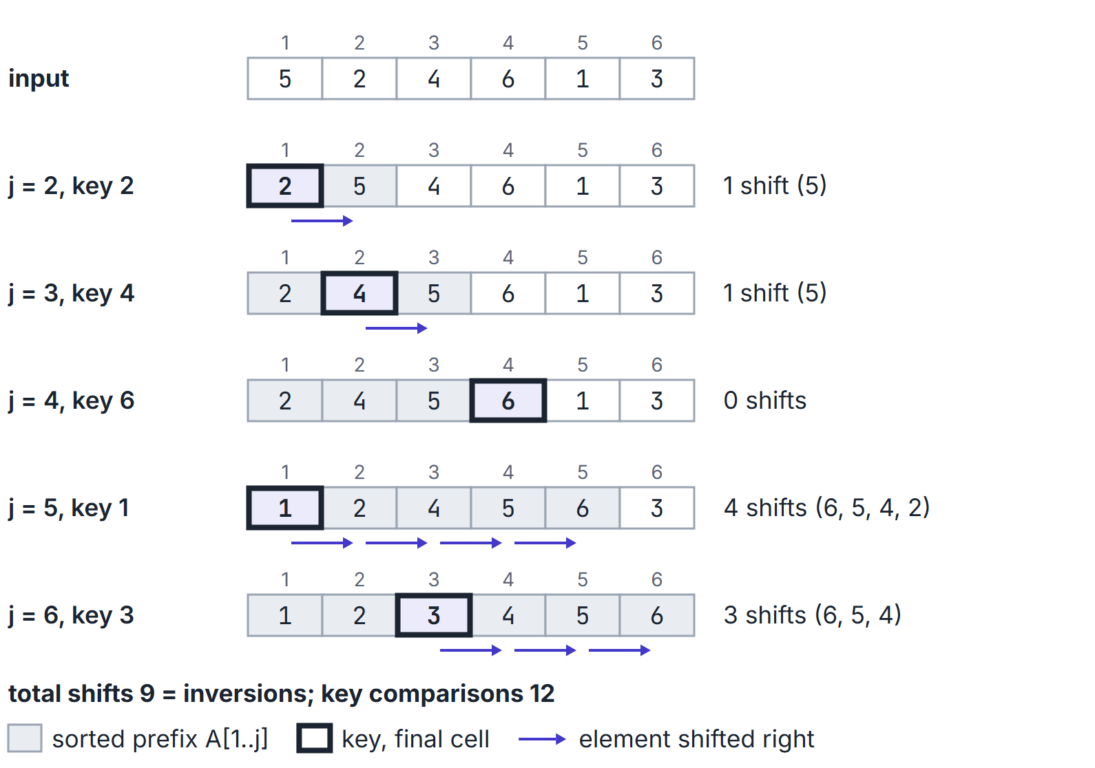
Analysis. Each shift removes exactly one inversion (the key passes one larger element), so the number of shifts equals . Each value of makes one extra comparison that stops the loop, unless the key reaches position 1. So the number of key comparisons lies between and ; in the trace, , because two keys (2 and 1) reached the front.
| Case | Input | Comparisons | Shifts | Time |
|---|---|---|---|---|
| Best | already sorted | 0 | ||
| Worst | strictly decreasing | |||
| Average | random order, distinct keys | about |
In general the running time is . Insertion sort is in place, stable (the strict test A[i] > key never moves a key past an equal one), adaptive and online.
Binary insertion sort finds the insertion point by binary search, cutting comparisons to in total. The shifts remain , so the worst-case time is still .
Selection sort
Idea. For , find the minimum of and exchange it into position .
SELECTION-SORT(A, n)
    for i <- 1 to n - 1
        min <- i
        for j <- i + 1 to n
            if A[j] < A[min] then min <- j
        if min != i then exchange A[i] with A[min]
Invariant. holds the smallest elements in sorted order.
Trace on : after : 1 2 4 6 5 3; : unchanged (2 is already the minimum); : 1 2 3 6 5 4; : 1 2 3 4 5 6; : unchanged. Comparisons 15, exchanges 3.
Analysis.
- Comparisons are always , whatever the input. Time is in the best, worst and average cases: selection sort is not adaptive.
- Exchanges: at most , the fewest of the three methods. This makes selection sort a reasonable choice when writing an element is much more expensive than comparing.
- In place.
- Not stable in the array form above. Example with keys compared by number only: . At the minimum 1 is exchanged with , giving ; the two 2s have changed order. A stable variant inserts the minimum by shifting instead of exchanging, at the cost of moves.
Bubble sort
Idea. Sweep left to right exchanging adjacent out-of-order pairs. Each pass moves the largest remaining element to the end, like a bubble rising. Stop early if a pass makes no exchange.
BUBBLE-SORT(A, n)
    for pass <- 1 to n - 1
        swapped <- FALSE
        for i <- 1 to n - pass
            if A[i] > A[i + 1]
                exchange A[i] with A[i + 1]
                swapped <- TRUE
        if swapped = FALSE then return
Invariant. After pass , the last positions hold the largest elements in their final order.
Trace on :
| Pass | Array after the pass | Comparisons | Exchanges |
|---|---|---|---|
| 1 | 2 4 5 1 3 6 | 5 | 4 |
| 2 | 2 4 1 3 5 6 | 4 | 2 |
| 3 | 2 1 3 4 5 6 | 3 | 2 |
| 4 | 1 2 3 4 5 6 | 2 | 1 |
| 5 | 1 2 3 4 5 6 | 1 | 0 |
Total: 15 comparisons and 9 exchanges .
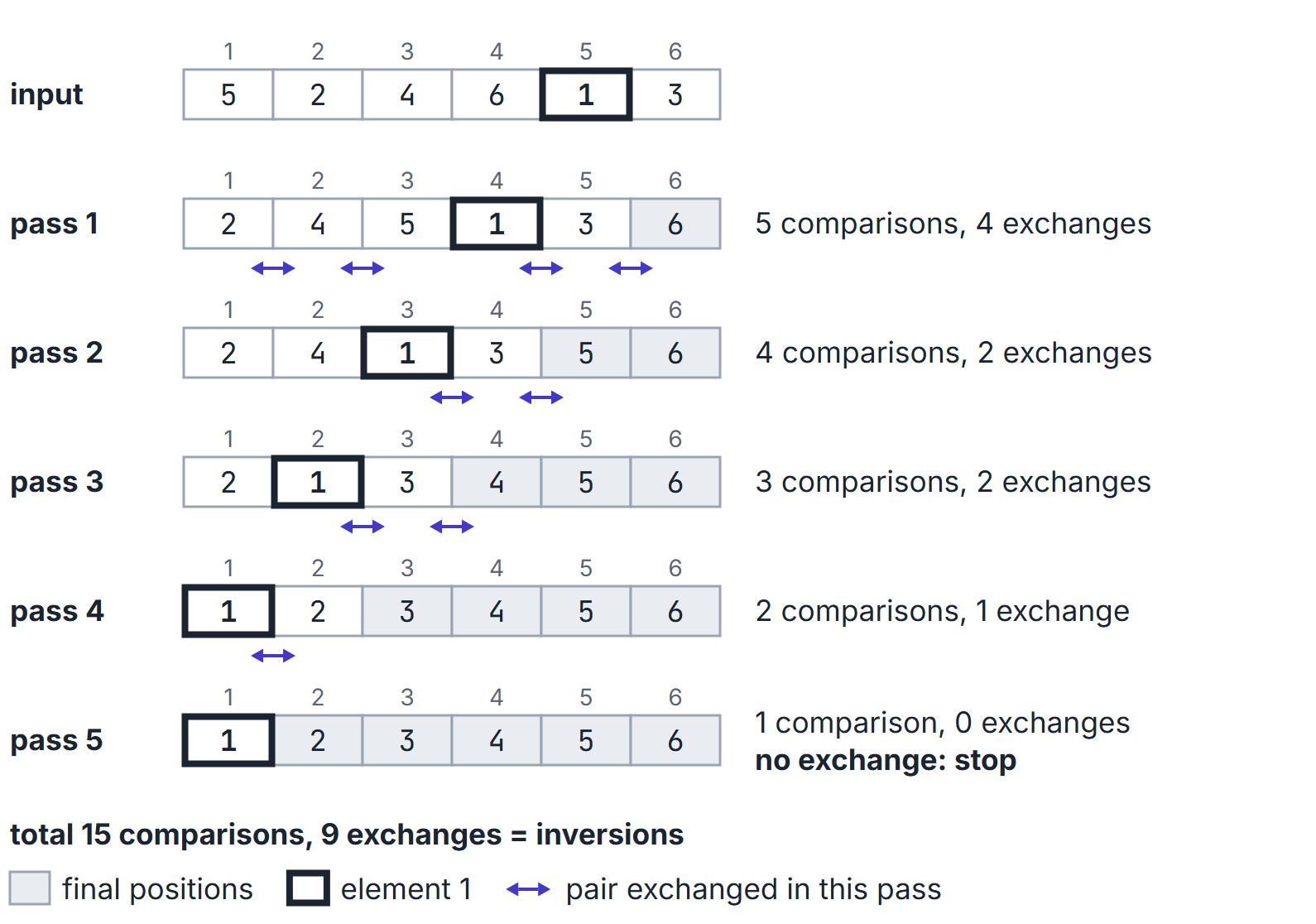
Analysis.
- Exchanges equal (each adjacent exchange removes one inversion).
- Passes. An element moves left by at most one position per pass. So the number of passes that make an exchange equals the largest number of greater elements to the left of any element. Here element 1 has four greater elements before it, so passes 1 to 4 exchange, and pass 5 confirms.
- With the
swappedflag: best case (sorted input) is one pass of comparisons, . Without the flag, bubble sort always makes comparisons. - Worst case (decreasing input): comparisons and exchanges, . Average .
- In place and stable (only strictly greater neighbours are exchanged).
A known asymmetry: a small element at the far right ("turtle") needs many passes to reach the front, while a large element at the far left ("rabbit") reaches the end in one pass.
Comparison
| Property | Bubble (with flag) | Selection | Insertion |
|---|---|---|---|
| Best-case time | |||
| Worst-case time | |||
| Average time | |||
| Comparisons, worst | (always) | ||
| Exchanges or shifts | at most | shifts | |
| Auxiliary space | |||
| Stable | yes | no (array form) | yes |
| Adaptive | yes | no | yes, |
| Online | no | no | yes |
Exact counts
- Insertion sort comparisons, exactly. The stopping comparison is missing only when the key becomes the new minimum, that is when is smaller than everything before it (a prefix minimum, ). So comparisons , where is the number of prefix minima at positions 2 to . In the trace, 2 and 1 are prefix minima: . On decreasing input every key is a prefix minimum, giving .
- Selection sort on decreasing input makes only exchanges, not . For 6 5 4 3 2 1: gives 1 5 4 3 2 6, gives 1 2 4 3 5 6, gives 1 2 3 4 5 6, and find the minimum already in place. Each exchange fixes two positions, the outer pair.
- Bubble sort passes, turtle against rabbit. With the flag, 2 3 4 5 6 1 takes 5 passes (the 1 moves one place per pass), while 6 1 2 3 4 5 takes 2 passes (the 6 reaches the end in pass 1, and pass 2 confirms). Both arrays have , so the exchange counts agree while the pass counts differ.
Edge cases
- or : all three loops do nothing useful and terminate; the array is trivially sorted.
- All keys equal: . Insertion sort and flagged bubble sort take ; selection sort still takes comparisons and makes no exchange (with the
min != itest). - Changing
>to>=in insertion sort or bubble sort destroys stability and adds useless moves of equal keys. - An array of distinct keys that becomes sorted when one element is moved positions has exactly inversions, so insertion sort sorts it in time.
Important properties and observations
- Any algorithm that exchanges only adjacent elements needs at least exchanges, so it is in the worst and average cases. Breaking the quadratic barrier requires moving elements over long distances (Shell sort, merge sort, quicksort, heapsort).
- Insertion sort is the method of choice for small and nearly sorted input; hybrid sorts switch to it below a small cut-off.
- Selection sort minimises writes; insertion sort minimises comparisons on nearly sorted data.
- After passes, bubble sort has placed the largest elements and selection sort the smallest; insertion sort has sorted the first elements (which need not be the smallest).
GATE examination perspective
- State after passes. Be precise about what each algorithm guarantees (largest at the end for bubble, smallest at the front for selection, sorted prefix of original elements for insertion).
- Counting. swaps of bubble sort and shifts of insertion sort equal the number of inversions; selection sort's comparisons are always .
- Stability and in-place questions. bubble and insertion are stable; array selection sort is not; all three are in place.
- Best case traps. bubble sort is only with the early-exit flag; selection sort is never better than .
- Exact-count traps. insertion sort comparisons are ; selection sort on decreasing input exchanges times; bubble sort passes depend on how far the smallest elements must travel left, not on .
Summary
Sources
- T. H. Cormen, C. E. Leiserson, R. L. Rivest, C. Stein, Introduction to Algorithms, 3rd ed., MIT Press, 2009: Section 2.1 (insertion sort and loop invariants), Section 2.2 (its analysis), Exercise 2.2-2 (selection sort), Problem 2-2 (bubble sort) and Problem 2-4 (inversions).