Collision Resolution: Chaining and Open Addressing

A hash function sends key $k$ to slot $h(k)$ of a table $T[0..m-1]$, and collisions (two keys with the same slot) cannot be avoided once the universe is larger than the table (see Hashing and Hash Functions). The cost analysis uses expectation and linearity of expectation from Random Variables, Expectation and Variance. A collision-resolution method decides where the second key goes and how a later search finds it.

There are two families. Chaining keeps a linked list in each slot, so a slot can hold any number of keys. Open addressing stores every key in the table itself and, on a collision, probes other slots in a fixed order until it finds a free one. This note gives the algorithms, traces all four standard methods on one input, and states the expected number of probes as a function of the load factor $\alpha = n/m$.

Slot $j$ holds a pointer to a linked list of all keys with $h(k) = j$ (NIL if there are none). New keys go at the head of their list.

Each slot holds one key, NIL (never used) or DELETED (used, then emptied). The hash function takes a second argument, the probe number $i = 0, 1, \ldots, m-1$:

is the probe sequence of $k$. INSERT takes the first slot in the sequence that is NIL or DELETED; SEARCH follows the same sequence until it finds $k$ or a NIL slot. For INSERT to succeed whenever the table has room, the probe sequence must be a permutation of $0, 1, \ldots, m-1$. Because all keys live in the table, $n \le m$ and so $\alpha \le 1$.

Let $h'$ (and $h_1$, $h_2$) be ordinary hash functions into $0..m-1$. For $m\ge2$, $\varphi(m)$ is Euler’s totient: the number of integers $d$ with $1\le d\le m-1$ and $\gcd(d,m)=1$. The three standard probe sequences are:

Primary versus secondary clustering. In linear probing, any key whose home slot falls anywhere inside an occupied run lands at the run's end and lengthens it, so long runs grow faster than short ones (primary clustering). In quadratic probing, only keys with the same home slot follow the same sequence (secondary clustering), which is milder. Double hashing gives keys with the same home different step sizes $h_2(k)$, so it avoids both.

Double hashing condition. The sequence visits every slot exactly when $\gcd(h_2(k), m) = 1$. Two standard ways: $m$ prime and $1 \le h_2(k) < m$, for example $h_2(k) = 1 + (k \bmod (m - 1))$; or $m$ a power of 2 and $h_2(k)$ always odd.

Quadratic probing may not visit every slot. With $h(k, i) = (h'(k) + i^2) \bmod m$ and $m = 11$, the offsets $i^2 \bmod 11$ for $i = 0, \ldots, 10$ take only the 6 values $0, 1, 4, 9, 5, 3$. With $m$ an odd prime, $i^2$ reaches exactly $(m+1)/2$ residues, so an insertion can fail even though the table has free slots. It is guaranteed to succeed while the table is at most half full.

Pseudocode uses 0-based slots $T[0..m-1]$, <- for assignment, x.key for the key of element x, and NIL and DELETED as markers.

INSERT is $O(1)$ worst case if it does not check for duplicates. DELETE is $O(1)$ worst case if it is given a pointer to the element and the lists are doubly linked (a singly linked list must first find the predecessor). SEARCH costs the length of one list.

Deletion leaves a marker. HASH-DELETE cannot set the slot to NIL: a later key whose probe sequence passed through this slot would then be cut off, because SEARCH stops at NIL. DELETED means "keep probing" to SEARCH and "free" to INSERT. With many deletions, search times depend on the number of markers as well as on $\alpha$, which is why chaining is preferred when keys are deleted often.

Counting convention. A probe is one examination of a slot. A successful first-try insertion or search costs 1 probe. In chaining, the cost of a search is the number of list elements compared, plus the $O(1)$ cost of computing $h$.

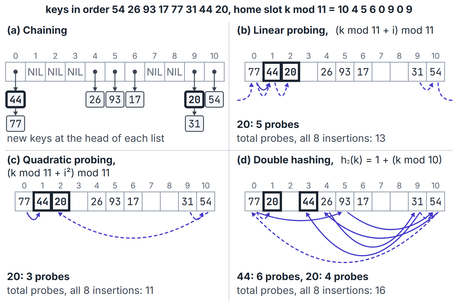
Insert $54, 26, 93, 17, 77, 31, 44, 20$, in that order, into a table with $m = 11$ and home slot $h'(k) = k \bmod 11$. The home slots are $10, 4, 5, 6, 0, 9, 0, 9$, so the first six keys go straight home and only 44 and 20 collide.

The details that decide exam answers:

After the linear-probing insertions the free slots are 3, 7 and 8. If the next key's home slot is uniformly random over $0..10$:

The free slot just after the longest run is the most likely target, so the run grows further. This is primary clustering in numbers.

A table of size 10 with $h'(k) = k \bmod 10$ and linear probing holds 42, 23, 34, 52, 46, 33 in slots 2 to 7, in that order, after six insertions into an empty table. Work out what each key needed when it was inserted.

So 33 is last, 52 follows 42, 23 and 34 (in any of $3! = 6$ orders), and 46 can go into any of the 5 positions among those four keys: $6 \times 5 = 30$ insertion orders produce the table. The order 46, 34, 42, 23, 52, 33 is one of them; 46, 42, 34, 52, 23, 33 is not (52 would take slot 3 before 23 arrived).

Expected bounds in this section assume insertion-only/no-tombstone occupancy models. With deletions, live load factor alone does not capture tombstone occupancy.

Let $\alpha = n/m$. The expected length of each list is $\alpha$.

because the keys examined before the target are those inserted after it into the same list, and each of the $n - 1$ other keys is in the target's list with probability $1/m$ and inserted after it in half the cases.

If $n = O(m)$, then $\alpha = O(1)$ and every chaining operation takes $O(1)$ expected time.

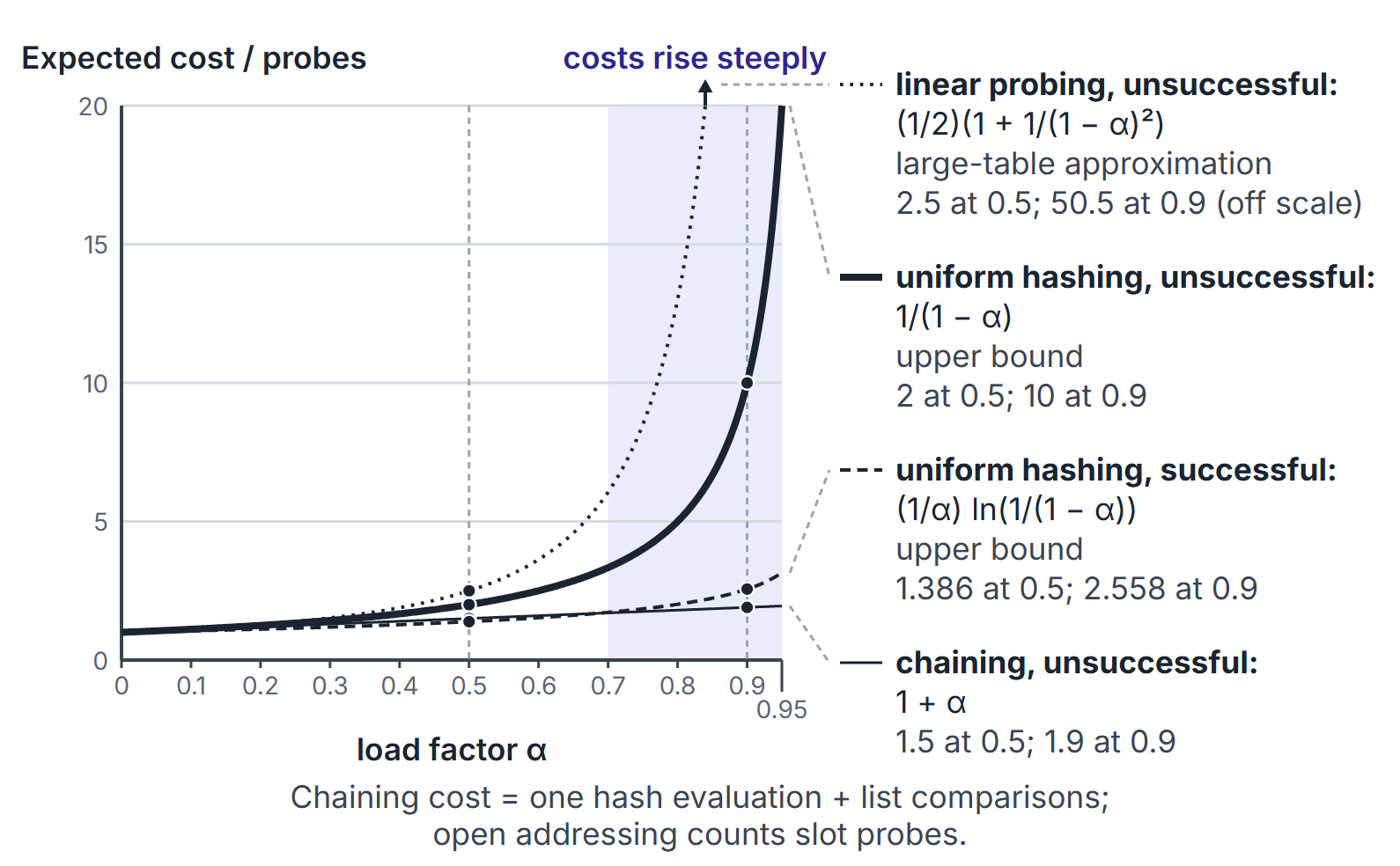
Uniform hashing assumes each key's probe sequence is equally likely to be any of the $m!$ permutations of $0..m-1$. For $\alpha < 1$, the expected number of probes is:

Why $1/(1 - \alpha)$. The first probe always happens. A slot is occupied with probability about $\alpha$, so a second probe happens with probability at most $\alpha$, a third with probability at most $\alpha^2$, and so on: $1 + \alpha + \alpha^2 + \cdots = 1/(1-\alpha)$. Inserting a key costs the same as an unsuccessful search for it. A successful search for the key inserted $(i+1)$-th repeats that insertion, which cost at most $1/(1 - i/m)$ probes; averaging over $i = 0..n-1$ and bounding the sum by an integral gives the logarithm.

Linear probing is worse. Linear probing cannot satisfy the uniform hashing assumption, because it has only $m$ probe sequences. Its standard analysis assumes instead that each key's home slot $h'(k)$ is uniformly random and independent of the others (simple uniform hashing of the home slot). Under that assumption, and because of primary clustering, the classical approximations for large $m$ are about $\frac{1}{2}\left(1 + \frac{1}{(1-\alpha)^2}\right)$ probes for an unsuccessful search and $\frac{1}{2}\left(1 + \frac{1}{1-\alpha}\right)$ for a successful one: 2.5 and 1.5 at $\alpha = 0.5$, but 50.5 and 5.5 at $\alpha = 0.9$. Double hashing behaves close to the uniform-hashing bounds.

Common misconceptions.