
Introduction
Quicksort sorts by divide and conquer, but puts the work in the divide step. It chooses a pivot, partitions the array so that smaller elements come before larger ones, and then sorts the two parts recursively; no combine step is needed. It sorts in place, and its average running time is with small constants, which is why it is often the fastest sort in practice. Its worst case, however, is , and the gap between the two cases is the centre of the analysis below.
Prerequisites
- Solving Recurrences and the Master Theorem: , , unequal splits.
- Elementary Sorting: stability and in-place.
- Expected value and indicator random variables, see Random Variables, for the average-case analysis.
The algorithm
Pseudocode uses 1-based arrays, <- for assignment and A[i..j] for the subarray from position to position .
QUICKSORT(A, p, r)
    if p < r
        q <- PARTITION(A, p, r)
        QUICKSORT(A, p, q - 1)
        QUICKSORT(A, q + 1, r)
Initial call: QUICKSORT(A, 1, n). After PARTITION, the pivot is at its final sorted position , every element of is , and every element of is (for the Lomuto scheme below).
Lomuto partition (CLRS 3e)
The pivot is the last element .
PARTITION(A, p, r)
    x <- A[r]
    i <- p - 1
    for j <- p to r - 1
        if A[j] <= x
            i <- i + 1
            exchange A[i] with A[j]
    exchange A[i + 1] with A[r]
    return i + 1
Invariant at the start of each iteration: , , not yet examined, .
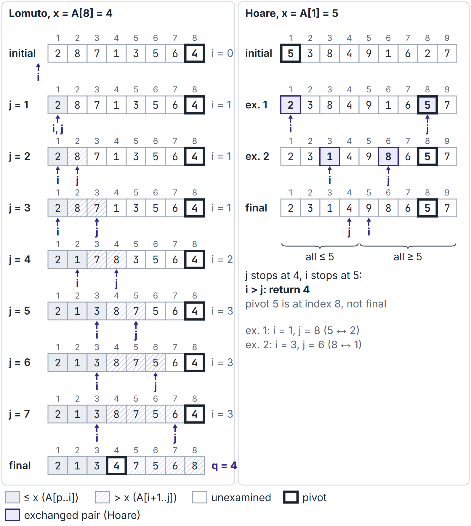
Trace on , pivot :
| ? | after | Array after the step | ||
|---|---|---|---|---|
| 1 | 2 | yes, exchange with itself | 1 | 2 8 7 1 3 5 6 4 |
| 2 | 8 | no | 1 | 2 8 7 1 3 5 6 4 |
| 3 | 7 | no | 1 | 2 8 7 1 3 5 6 4 |
| 4 | 1 | yes, exchange , | 2 | 2 1 7 8 3 5 6 4 |
| 5 | 3 | yes, exchange , | 3 | 2 1 3 8 7 5 6 4 |
| 6 | 5 | no | 3 | 2 1 3 8 7 5 6 4 |
| 7 | 6 | no | 3 | 2 1 3 8 7 5 6 4 |
| final | exchange , | 2 1 3 4 7 5 6 8 |
PARTITION returns . It makes exactly key comparisons, for a subarray of elements, on every input. It executes the exchange line 4 times (at , 4 and 5, plus the final one); if exchanges of an element with itself are not counted, that is 3. Questions that ask for "the number of swaps" usually intend one of these two conventions, so check which.
Hoare partition
The pivot is the first element ; two indices move towards each other and exchange out-of-place pairs.
HOARE-PARTITION(A, p, r)
    x <- A[p]
    i <- p - 1
    j <- r + 1
    while TRUE
        repeat j <- j - 1 until A[j] <= x
        repeat i <- i + 1 until A[i] >= x
        if i < j then exchange A[i] with A[j]
        else return j
With Hoare partition the recursive calls are QUICKSORT(A, p, j) and QUICKSORT(A, j + 1, r). It guarantees every element of is every element of , but the pivot is not necessarily at its final position, and is not the pivot's index.
Trace on , : first stops at 8 () and at 1 (); exchange to get 2 3 8 4 9 1 6 5 7. Next stops at 6 (value 1) and at 3 (value 8); exchange to get 2 3 1 4 9 8 6 5 7. Next stops at 4 (value 4) and at 5 (value 9); now , so return . The parts are and ; the pivot 5 sits inside the right part.
Hoare's scheme makes about three times fewer exchanges than Lomuto's on average and handles many equal keys far better, because both indices stop on keys equal to the pivot.
Analysis
Let be the time on elements. Partition costs . If it produces parts of sizes and :
Worst case:
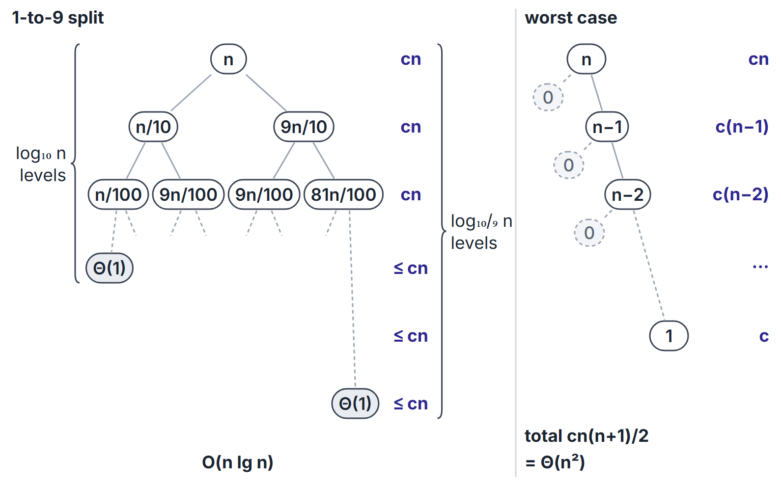
The worst split is and at every level: . With the last-element pivot this happens on already sorted input, on reverse-sorted input, and (for Lomuto) on input where all keys are equal. The number of comparisons is then , and the recursion depth is .
Best case:
For distinct keys, if every pivot is the median, .
Any constant-proportion split:
Even a persistently lopsided split such as 1 to 9 gives . The recursion tree has full levels of cost at most and depth , so . Only splits that are lopsided by a non-constant factor, such as a constant number of elements on one side, cause quadratic time.
Average case:
For the shown Lomuto partition, assume distinct keys throughout this randomized analysis. Assume all orderings of distinct keys are equally likely, or use randomized quicksort, which picks the pivot uniformly at random from (exchange it with , then run PARTITION). Let be the keys in sorted order. Two keys are compared at most once, only when one of them is the first pivot chosen from , which happens with probability . Summing over all pairs,
where is the -th harmonic number. For randomized quicksort this expectation holds for every input of distinct keys: no particular input is bad, only unlucky random choices are, and they are very unlikely.
Small cases make the formula concrete. For it gives , and for it gives ; averaging Lomuto quicksort's comparison count over all 6 (or 24) input orders gives exactly these values. The pair probability is useful on its own: adjacent keys are always compared (probability ), since no key between them can separate them, while the smallest and largest keys are compared with probability only (one of them must be the very first pivot).
Space
Quicksort uses auxiliary space besides the recursion stack, so it is called in place. The stack depth is on balanced splits but in the worst case. Recursing on the smaller part first and looping on the larger (tail-call elimination) bounds the depth by in every case.
Summary of cases
| Case | When (last-element pivot) | Comparisons | Time | Stack depth |
|---|---|---|---|---|
| Best | distinct keys; pivot is always the median | about | ||
| Average or randomized | distinct keys: random order, or random pivot | expected | ||
| Worst | sorted, reverse sorted, or all equal (Lomuto) |
Properties and practical improvements
- Not stable. Long-distance exchanges reorder equal keys. Example with Lomuto: partitions around pivot 1 to give .
- In place (apart from the stack) and not adaptive: sorted input is the worst case for the naive pivot choice.
- Pivot choice. Random pivot, or median-of-three (median of first, middle and last), avoids the sorted-input worst case. With distinct keys for this partition, choosing the exact median with the linear-time selection algorithm guarantees in the worst case but is slow in practice.
- Many equal keys. A three-way partition (Dutch national flag) splits into , and and does not recurse on the middle part, so an all-equal array takes .
- Small subarrays. Switching to insertion sort below a small cut-off saves time.
- Hybrids. Introsort runs quicksort but switches to heapsort if the recursion becomes too deep, keeping the worst case at .
Quickselect: the $k$-th smallest element
Related material. Selection is not a separate item of the GATE syllabus. It is included because it reuses PARTITION and is commonly studied together with quicksort.
The same partition finds the -th smallest element without sorting: partition, then recurse into one side only.
QUICKSELECT(A, p, r, k)          // distinct keys; k-th smallest of A[p..r], 1 <= k <= r - p + 1
    if p = r then return A[p]
    q <- RANDOMIZED-PARTITION(A, p, r)
    m <- q - p + 1                 // rank of the pivot within A[p..r]
    if k = m then return A[q]
    else if k < m then return QUICKSELECT(A, p, q - 1, k)
    else return QUICKSELECT(A, q + 1, r, k - m)
For distinct keys, the displayed Lomuto-based Quickselect has expected time (the expected sizes shrink geometrically) and worst case . The median-of-medians pivot rule (groups of 5) gives worst-case under the same distinct-key condition. To retain these linear guarantees with duplicate keys, use a three-way partition and return immediately when k lies in the equal block (CLRS 3e, Section 9.3).
Quickselect time and workspace. Here , comparisons, swaps and random-index generation are constant-time, and each pivot is chosen uniformly in the current subarray. Best time is , when the first partition finds the target. Without tail-call elimination, the displayed one-subproblem recursion has best call-stack space, expected space and worst space, with constant-size frames and no copied subarrays; input storage and the scalar result are excluded. Replacing the single recursive call by a loop gives auxiliary words with the same time bounds. These randomized stack bounds do not analyze the median-of-medians pivot subroutine; a straightforward implementation that copies medians into separate arrays uses auxiliary words including its stack.
Edge cases
- or :
p < ris false; nothing happens. - Two elements: one partition with one comparison.
- All keys equal: Lomuto puts everything on the left (every ), producing the worst case; Hoare splits near the middle.
- Lomuto partitions on the last element. Questions that say "first element as pivot" mean a variant: exchange with first, or use Hoare's scheme; check which.
Important properties and observations
- After one Lomuto partition, the pivot is in its final position; after a Hoare partition, that is not guaranteed.
- The number of comparisons in one Lomuto partition of elements is always .
- Worst-case recurrence ; best ; 1-to- split for constant still gives .
- Randomization changes the guarantee from "average over inputs" to "expected for every input of distinct keys (for the shown partition)".
GATE examination perspective
- Partition traces. the array after the first partition, the pivot's final index, or the number of exchanges. State the scheme (Lomuto or Hoare) and the pivot position before tracing.
- Worst-case recognition. sorted or reverse-sorted input with first or last pivot; all-equal keys with Lomuto.
- Probability questions. and are compared with probability : 1 for neighbours in sorted order, for the minimum and maximum.
- Recurrences for given splits. "the pivot always splits off elements" gives ; "the pivot always leaves 5 elements on one side" gives .
- Properties. in place, not stable, average , worst , stack when the smaller side is recursive and the larger side is iterative.
Summary
Sources
- T. H. Cormen, C. E. Leiserson, R. L. Rivest, C. Stein, Introduction to Algorithms, 3rd ed., MIT Press, 2009, Chapter 7 (Sections 7.1 to 7.4: PARTITION, performance, randomized quicksort and its expected-comparison analysis; Problem 7-1 on Hoare partition; Problem 7-4 on stack depth) and Chapter 9 (Sections 9.2 and 9.3: randomized and worst-case linear-time selection).