
Introduction
Three classical DP problems share a tabular fill and a reconstruction step: the 0/1 knapsack problem (and its decision twin subset sum), and matrix-chain multiplication. Density order solves the fractional knapsack but fails for 0/1; matrix-chain parenthesization has no useful greedy rule either (CLRS Exercise 15.3-4). Both need DP.
This note states the recurrences, works a full knapsack table and a small matrix-chain table, and records the standard complexities and .
Prerequisites
- Dynamic Programming Fundamentals: state, transition, bottom-up fill, reconstruction.
- Greedy Algorithms: why density order fails for 0/1 knapsack.
Core concepts
0/1 knapsack
Input. items with weights and values , capacity . Each item is taken wholly or not at all.
State. Let be the maximum value using a subset of the first items with total weight at most .
Answer . Time and space (pseudo-polynomial in the numeric magnitude of ).
Subset sum
Decision version. Given positive integers and target , does a subset sum to ? Same table with values replaced by booleans (or by 0/1): item with weight and value , capacity ; accept if . The optimisation version (subset of sum closest to without exceeding) is the knapsack table with .
Matrix-chain multiplication
Input. Dimensions for matrices with of size .
Goal. Fully parenthesize the product to minimise the number of scalar multiplications. Multiplying an matrix by a matrix costs .
State. Let be the minimum cost of computing , and let be an optimal split index.
Number of states ; each state tries splits: time. The number of full parenthesizations is the Catalan number , which is exponential, so enumeration is hopeless.
Algorithms and pseudocode
Pseudocode uses 1-based arrays, <- for assignment and A[i..j] for the subarray from position to position .
0/1 knapsack
Preconditions: and all are integers; denotes the weight array, never a loop counter.
ZERO-ONE-KNAPSACK(v, w, W, n)
 1  let V[0..n, 0..W] be a new table
 2  for wt <- 0 to W
 3      V[0, wt] <- 0
 4  for i <- 1 to n
 5      V[i, 0] <- 0
 6      for wt <- 1 to W
 7          V[i, wt] <- V[i - 1, wt]
 8          if w[i] <= wt then
 9              V[i, wt] <- max(V[i, wt], v[i] + V[i - 1, wt - w[i]])
10  return V[n, W]
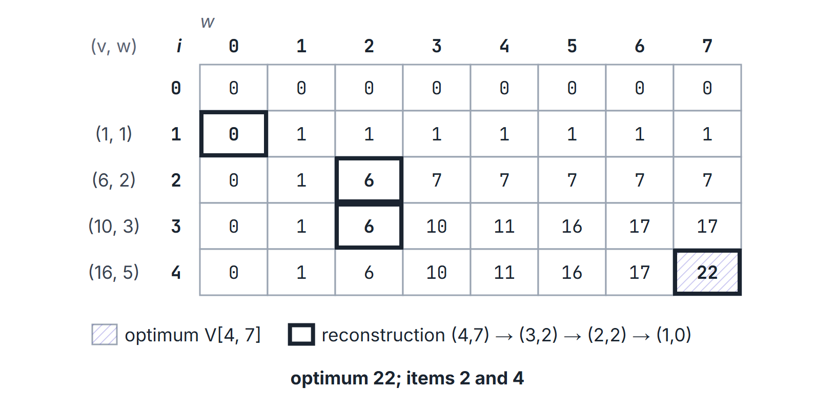
Reconstruction. From : if then item is unused, step to ; otherwise item is used, emit and step to .
Space. Only the previous row is needed for the value: extra space. Reconstruction then needs either the full table or a separate choice bit per cell.
One-array version: the direction of the inner loop matters. With a single array d[0..W] updated as d[wt] <- max(d[wt], v[i] + d[wt - w[i]]), scan wt downward from to for 0/1 knapsack. Then d[wt - w[i]] still holds the value from row , so item is used at most once. Scanning upward reads values already updated in row and silently solves the unbounded knapsack instead. On the four-item example below, the upward scan gives 20 at capacity 6 (item 3 taken twice) where the 0/1 answer is 17.
Edge cases. or returns 0. Items with are never taken. Ties do not affect the optimal value. They do affect which subset is reported: the reconstruction rule above treats item as unused whenever , so on a tie it prefers to exclude. State the tie-break if a question asks which subset.
Matrix-chain order
MATRIX-CHAIN-ORDER(p)
 1  n <- p.length - 1
 2  let m[1..n, 1..n] and s[1..n, 1..n] be new tables
 3  for i <- 1 to n
 4      m[i, i] <- 0
 5  for ell <- 2 to n                    // chain length
 6      for i <- 1 to n - ell + 1
 7          j <- i + ell - 1
 8          m[i, j] <- infinity
 9          for k <- i to j - 1
10              q <- m[i, k] + m[k + 1, j] + p[i - 1] * p[k] * p[j]
11              if q < m[i, j] then
12                  m[i, j] <- q
13                  s[i, j] <- k
14  return (m, s)
Time / space. time, space. Fill by increasing chain length ell so that every shorter chain is already known.
Printing the parenthesization. Recursively: if print ; else print ( + chain + chain + ).
Exact counts. The table has non-trivial cells with . Line 10 runs once per pair and split , that is times. For : 6 cells and 10 evaluations of .
Cost model. Multiplying a matrix by a matrix with the standard method takes scalar multiplications (and additions) and yields a matrix. Matrix-chain questions count multiplications only.
Mathematical explanation
Optimal substructure for knapsack
In any optimal packing of capacity using items , item is either absent (then the packing is optimal for ) or present (then the rest is optimal for ). Those are the only two options, so the recurrence is exhaustive.
Why density greedy fails
Items , . Densities 6, 5, 4. Greedy-by-density for 0/1 takes the first two (value 160) and cannot fit the third; the optimum is items 2 and 3 (value 220). The fractional optimum on the same instance is 240 (Greedy Algorithms).
Optimal substructure for matrix-chain
An optimal parenthesization of splits at some into and . Each side must itself be optimally parenthesized, otherwise a cheaper side could replace it. Minimising over yields (CLRS 3e, Section 15.2).
Catalan bound
The number of ways to parenthesize matrices is . For , ; for , . DP evaluates each of the subchains once instead of enumerating trees.
Worked examples
0/1 knapsack, four items
Items : ; . Index items 1..4 in that order.
Final row equals . Optimum 22: items 2 and 4 (weights , values ), or check by reconstruction from : and , so items 4 and 2.
Selected cells used in the figure:
| 0 | 1 | 2 | 3 | 4 | 5 | 6 | 7 | |
|---|---|---|---|---|---|---|---|---|
| 0 | 0 | 0 | 0 | 0 | 0 | 0 | 0 | 0 |
| 1 | 0 | 1 | 1 | 1 | 1 | 1 | 1 | 1 |
| 2 | 0 | 1 | 6 | 7 | 7 | 7 | 7 | 7 |
| 3 | 0 | 1 | 6 | 10 | 11 | 16 | 17 | 17 |
| 4 | 0 | 1 | 6 | 10 | 11 | 16 | 17 | 22 |
Matrix-chain on four matrices
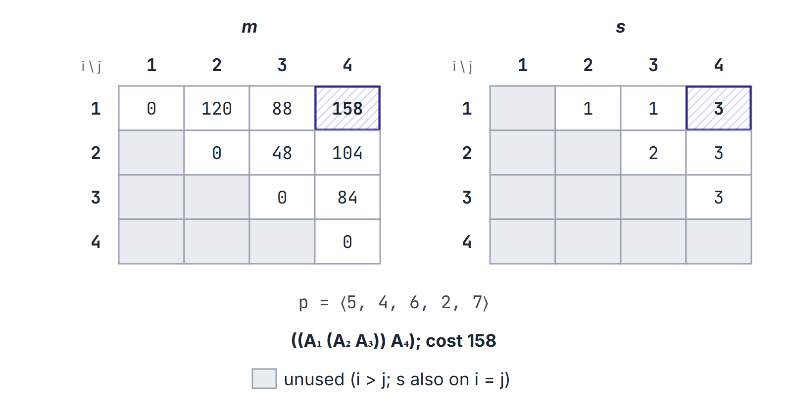
Dimensions (matrices , , , ).
Chain length 2:
- ,
- ,
- ,
Chain length 3:
- ,
- ,
Chain length 4:
- , .
Optimal cost 158 with split : . Expanding with gives .
All parenthesizations, for comparison:
| Parenthesization | Cost |
|---|---|
| 158 | |
| 244 | |
| 250 | |
| 392 | |
| 414 |
The worst order costs more than 2.6 times the best. Plain left-to-right evaluation (250) is not optimal here.
Important properties and observations
- 0/1 knapsack is pseudo-polynomial: is polynomial in and , not in the bit length of . The decision version is NP-complete, so no algorithm polynomial in the input size is expected unless P = NP.
- Unbounded knapsack (unlimited copies of each item) changes the transition to (same-row reuse). Do not mix the two recurrences. For the four-item example, the unbounded optimum by capacity is : capacity 4 gives 12 (item 2 twice) against 11 for 0/1.
- Increasing chain length is one convenient valid matrix-chain fill order. Ordinary top-to-bottom row-major order is invalid. Another valid order is rows i=n down to 1, with columns j=i+1 up to n: both required subchains are then already computed.
- The split table stores one optimal ; several may share the same cost.
Common misconceptions.
- "Knapsack is like fractional." Only the fractional version is greedy.
- "Matrix-chain needs parenthesizations." The count is Catalan, still exponential, which is why DP helps.
- "Subset sum needs values different from weights." Setting reduces knapsack to subset sum.
GATE examination perspective
- FILL ONE ROW. A question may give a partially filled knapsack table; compute the next cell from the recurrence.
- PSEUDO-POLYNOMIAL. State , not "polynomial" without qualification.
- CHAIN LENGTH ORDER. Matrix-chain questions ask for or after a few lengths.
- PARENTHESES COUNT. ways; DP cost .
- RECONSTRUCTION. Be ready to list which items are taken or to write the parenthesization from .
- ONE-ARRAY LOOP DIRECTION. Downward for 0/1, upward for unbounded; a question may show code and ask which problem it solves.
- MULTIPLICATION COUNT. per product; compare every parenthesization only when the chain is short (5 orders for 4 matrices, 14 for 5).
Summary
Sources
- T. H. Cormen, C. E. Leiserson, R. L. Rivest, C. Stein, Introduction to Algorithms, 3rd ed., MIT Press, 2009: Chapter 15, Section 15.2 (matrix-chain multiplication) and Section 15.3 (elements of dynamic programming); Exercise 15.3-4 (greedy split fails).