Merge Sort: short notes (Algorithms)

Introduction

Merge sort is the standard example of divide and conquer. It splits the array into two halves, sorts each half recursively, and merges the two sorted halves in linear time. Its worst-case running time is $\Theta(n \lg n)$ , which matches the lower bound for comparison sorting, and it is stable. Its main cost is $\Theta(n)$ auxiliary memory for merging arrays. It is the usual choice for sorting linked lists and for external sorting of data that does not fit in memory.

Prerequisites

Solving Recurrences and the Master Theorem: $T(n) = 2T(n/2) + \Theta(n)$ .
Elementary Sorting: stability, in-place, inversions.

The merge procedure

Purpose. Combine two adjacent sorted subarrays $A[p..q]$ and $A[q+1..r]$ into one sorted subarray $A[p..r]$ . Precondition. $p \le q < r$ , and both subarrays are sorted.

Pseudocode uses 1-based arrays, <- for assignment and A[i..j] for the subarray from position $i$ to position $j$ .

Text

MERGE(A, p, q, r)
    L <- copy of A[p..q]           // n1 = q - p + 1 elements
    R <- copy of A[q+1..r]         // n2 = r - q elements
    i <- 1;  j <- 1;  k <- p
    while i <= n1 and j <= n2
        if L[i] <= R[j]
            A[k] <- L[i];  i <- i + 1
        else
            A[k] <- R[j];  j <- j + 1
        k <- k + 1
    copy the rest of L[i..n1], then the rest of R[j..n2], into A[k..r]

CLRS 3e places a sentinel $\infty$ at the end of $L$ and $R$ instead of testing for exhaustion; the result is the same.

Why <= matters. On a tie the element from the left half is taken first. Since left-half elements came earlier in the input, equal keys keep their order: this is what makes merge sort stable. Using < would break stability.

Cost of one merge of $n_1$ and $n_2$ elements:

Moves: exactly $n_1 + n_2$ (plus the copy into $L$ and $R$ ).
Key comparisons: at least $\min(n_1, n_2)$ (one list runs out after all its elements are taken, each after a comparison) and at most $n_1 + n_2 - 1$ (every output except the last needs a comparison).
Time $\Theta(n_1 + n_2)$ ; auxiliary space $\Theta(n_1 + n_2)$ .

The algorithm

Text

MERGE-SORT(A, p, r)
    if p < r
        q <- floor((p + r) / 2)
        MERGE-SORT(A, p, q)
        MERGE-SORT(A, q + 1, r)
        MERGE(A, p, q, r)

Initial call: MERGE-SORT(A, 1, n). A subarray of one element ( $p = r$ ) is already sorted.

Worked example

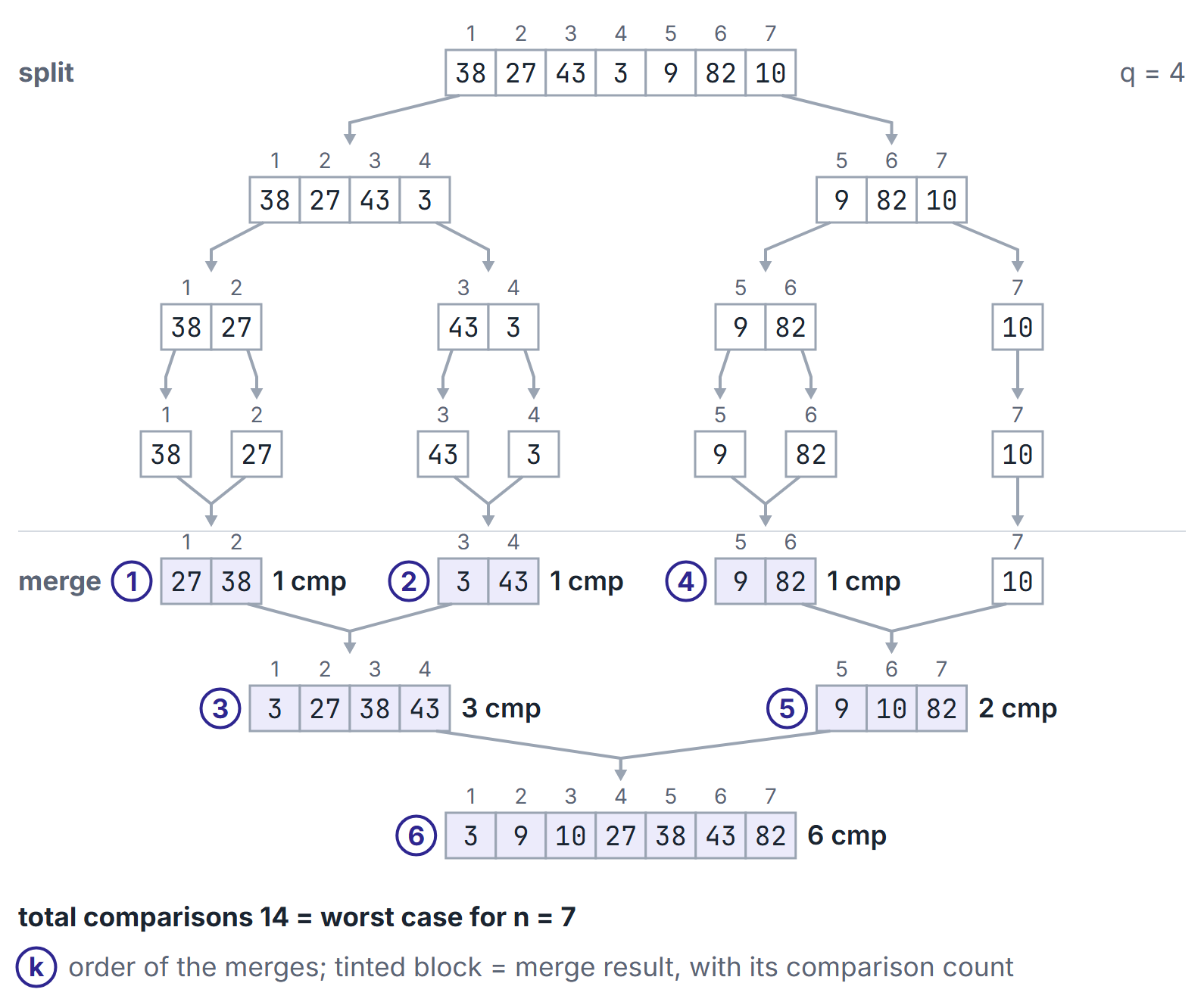
Input $A = [38, 27, 43, 3, 9, 82, 10]$ , $n = 7$ . The split points are $q = 4$ for $[1..7]$ , then $q = 2$ and $q = 6$ , and so on. The merges happen in this order:

Merge	Left	Right	Result	Comparisons
$A[1..2]$	38	27	27 38	1
$A[3..4]$	43	3	3 43	1
$A[1..4]$	27 38	3 43	3 27 38 43	3
$A[5..6]$	9	82	9 82	1
$A[5..7]$	9 82	10	9 10 82	2
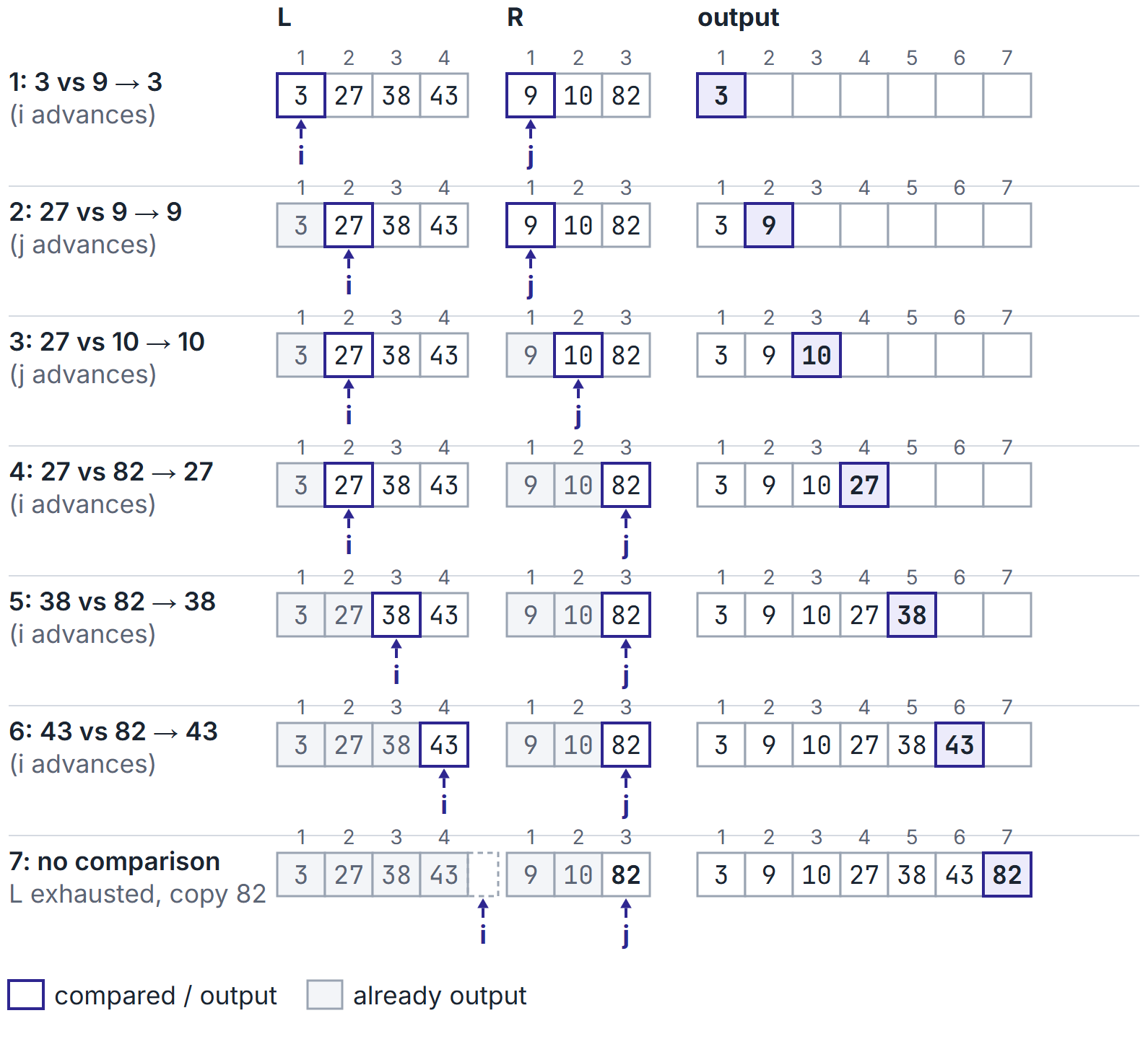
$A[1..7]$	3 27 38 43	9 10 82	3 9 10 27 38 43 82	6

Total: 14 key comparisons. This happens to be the worst case for $n = 7$ (formula below).

Merge sort split and merge tree — Figure 1. Merge sort on 38 27 43 3 9 82 10: the top half splits the array down to single elements; the bottom half merges them back, each merged block labelled with its comparison count.

The final merge step by step — Figure 2. The final merge of 3 27 38 43 with 9 10 82: pointers $i$ and $j$ , the element output at each of the 6 comparisons, and the leftover 82 copied without comparison.

Analysis

Running time

The divide step is $\Theta(1)$ , the two recursive calls cost $2T(n/2)$ , and merging costs $\Theta(n)$ :

T(n) = 2T(n/2) + \Theta(n), \qquad T(1) = \Theta(1).

By case 2 of the master theorem, $T(n) = \Theta(n \lg n)$ . For $n$ a power of two, the full recursion levels each do $\Theta(n)$ work. For general $n$ , there are $O(\lg n)$ levels with $O(n)$ work per level, and $\Theta(\lg n)$ full internal levels supply the matching lower bound.

The bound holds in every case. Merge sort does the same splits and the same amount of copying on every input of size $n$ ; only the number of comparisons inside the merges depends on the data.

Case	Time	Key comparisons (exact, for the top-down version above)
Best	$\Theta(n \lg n)$	$\tfrac{n}{2} \lg n$ when $n$ is a power of 2 (for example, already sorted input)
Worst	$\Theta(n \lg n)$	$n \lceil \lg n \rceil - 2^{\lceil \lg n \rceil} + 1$
Average	$\Theta(n \lg n)$	$n \lg n - \Theta(n)$

The worst-case formula gives 0, 1, 3, 5, 8, 11, 14 for $n = 1, \ldots, 7$ , and $n \lg n - n + 1$ when $n$ is a power of 2 (for example 17 for $n = 8$ ).

Space

Auxiliary arrays for merging: $\Theta(n)$ (at most $n$ elements are copied at any time if the buffers are freed after each merge, or one buffer of size $n$ is reused).
Recursion stack: $\Theta(\lg n)$ .
Total auxiliary space $\Theta(n)$ . Standard array merge sort is therefore not in place. (In-place merging algorithms exist but are complicated and slower in practice.)

Properties

Property	Merge sort
Time, all cases	$\Theta(n \lg n)$
Auxiliary space	$\Theta(n)$ for arrays; $\Theta(\lg n)$ stack only for linked lists
Stable	yes (take from the left half on ties)
In place	no (array version)
Adaptive	no (standard version)
Comparison-based	yes, and asymptotically optimal

Variants

Bottom-up (iterative) merge sort

Treat the array as $n$ runs of length 1. Merge adjacent pairs of runs to get runs of length 2, then 4, and so on. There are $\lceil \lg n \rceil$ passes, each $\Theta(n)$ , and no recursion. For $n = 7$ : passes of run length 1, 2 and 4, so $\lceil \lg 7 \rceil = 3$ passes. The merge pattern differs from top-down merge sort when $n$ is not a power of 2, so exact comparison counts can differ.

On the worked example the array after each pass is:

Pass	Run length merged	Array after the pass	Comparisons
1	1	27 38 3 43 9 82 10	3
2	2	3 27 38 43 9 10 82	5
3	4	3 9 10 27 38 43 82	6

The lone 10 waits unmerged in pass 1. Here the total is also 14 comparisons, but the intermediate arrays differ from the top-down order: top-down finishes $A[1..4]$ before it touches $A[5..7]$ , while bottom-up treats the whole array level by level. A question about "the array after the second pass" means bottom-up.

Natural merge sort

Start from the maximal already-sorted runs of the input instead of runs of length 1. On sorted input there is one run and the sort takes $\Theta(n)$ time; this makes it adaptive.

Linked lists

Splitting a list (find the middle with slow and fast pointers) and merging two sorted lists need only pointer changes, so merge sort sorts a linked list in $\Theta(n \lg n)$ time with only the $\Theta(\lg n)$ recursion stack as extra space (or $O(1)$ bottom-up). Classic array-based heapsort needs random access and is a poor fit for lists. Quicksort can partition a linked list in linear time, but retains pivot/balance risks and is not stable in its usual form; merge sort is the natural stable choice. See Linked Lists.

$k$ -way merging and external sorting

Merging $k$ sorted lists with $n$ elements in total, using a min-heap of the $k$ current front elements, takes $O(n \lg(k+1))$ time. External sorting writes sorted runs to disk and then merges them in a few $k$ -way passes, so that each pass reads the data sequentially.

Small-subarray cut-off

Practical implementations switch to insertion sort for subarrays below a small size, because insertion sort has lower overhead on tiny inputs.

Applications of merging

Counting inversions in $\Theta(n \lg n)$ : during a merge, when an element $R[j]$ is output while $L[i..n_1]$ remain, it forms $n_1 - i + 1$ inversions with them. Summing over all merges counts every inversion exactly once. For $[38, 27, 43, 3, 9, 82, 10]$ the count is 11.
Union and intersection of two sorted lists in linear time.
Merging two sorted arrays of sizes $m$ and $n$ : $m + n - 1$ comparisons in the worst case, $\min(m, n)$ in the best.
Merging several sorted lists two at a time. The order of the pairwise merges matters. For lists of sizes 20, 24, 30, 35 and 50, merging in the given order costs $(20 + 24 - 1) + (44 + 30 - 1) + (74 + 35 - 1) + (109 + 50 - 1) = 382$ comparisons in the worst case. Always merging the two smallest lists first (20 with 24, 30 with 35, 44 with 50, then 65 with 94) costs $43 + 64 + 93 + 158 = 358$ , the minimum. This is the greedy optimal merge pattern, with $a + b - 1$ comparisons per merge instead of $a + b$ moves.

Edge cases

$n = 0$ or $n = 1$ : no work; the base case $p \ge r$ returns.
All keys equal: every merge takes all of $L$ first (ties go left), using $n_1$ comparisons; stability is preserved.
Odd sizes: with $q = \lfloor (p + r)/2 \rfloor$ the left half gets the extra element.
Overflow of $p + r$ in fixed-width integers: compute $q = p + \lfloor (r - p)/2 \rfloor$ .

Important properties and observations

The $\Theta(n \lg n)$ bound does not depend on the input order, unlike quicksort's.
Merge sort is optimal in the comparison model up to lower-order terms: its worst case $n \lg n - \Theta(n)$ comparisons is close to $\lg(n!) \approx n \lg n - 1.44n$ .
The number of merges is $n - 1$ (each merge reduces the number of runs by one), and the number of calls to MERGE-SORT is $2n - 1$ .
Merge sort is the basis of stable library sorts for objects (for example, Timsort is a natural merge sort with insertion-sort runs).

GATE examination perspective

Comparison counts. best and worst numbers of comparisons to merge two sorted lists ( $\min(m, n)$ and $m + n - 1$ ); the worst-case count of the whole sort for a small $n$ .
Intermediate states. the array after a given number of merges or passes; follow the recursion order (left subtree first) for top-down, level by level for bottom-up.
Several lists. worst-case comparisons for merging many sorted lists pairwise: merge the two smallest first, $a + b - 1$ per merge.
Recurrence questions. variants such as splitting into three parts ( $3T(n/3) + \Theta(n)$ , still $\Theta(n \lg n)$ ) or merging in $\Theta(n^2)$ time ( $2T(n/2) + \Theta(n^2) = \Theta(n^2)$ ).
Property questions. stable, not in place, $\Theta(n \lg n)$ in all cases, best for linked lists.

Summary

Solving Recurrences and the Master Theorem: prerequisite. Case 2 of the master theorem.
Divide and Conquer: related. The paradigm and other examples.
Quicksort: related. Divide and conquer with the work in the divide step instead of the combine step.
Comparison of Sorting Algorithms: dependent. Merge sort against the other sorts and the lower bound.
Binary Heaps: related. Used in $k$ -way merging.

Merge Sort

Introduction

Prerequisites

The merge procedure

The algorithm

Worked example

Analysis

Running time

Space

Properties

Variants

Bottom-up (iterative) merge sort

Natural merge sort

Linked lists

$k$ -way merging and external sorting

Small-subarray cut-off

Applications of merging

Edge cases

Important properties and observations

GATE examination perspective

Summary

Sources

Next steps

Introduction

Prerequisites

The merge procedure

The algorithm

Worked example

Analysis

Running time

Space

Properties

Variants

Bottom-up (iterative) merge sort

Natural merge sort

Linked lists

kkk-way merging and external sorting

Small-subarray cut-off

Applications of merging

Edge cases

Important properties and observations

GATE examination perspective

Summary

Related topics

Sources

Next steps

$k$ -way merging and external sorting