
Introduction
Every comparison sort needs comparisons in the worst case (see Comparison of Sorting Algorithms). The three algorithms in this note beat that bound because they are not comparison sorts: they use the keys as array indices or split them into digits. Each works only under an assumption about the keys:
| Algorithm | Assumption on keys | Time |
|---|---|---|
| Counting sort | integers in | |
| Radix sort | digits, each in | |
| Bucket sort | real numbers drawn uniformly from | expected |
When and is a constant, all three are linear.
Prerequisites
- Elementary Sorting: stability (essential here) and insertion sort (used inside bucket sort).
- Arrays with 1-based indexing; counting arrays are indexed from 0.
Counting sort
Purpose. Sort integers in the range stably. Input. with . Output. , a sorted copy. Auxiliary: .
Pseudocode uses 1-based arrays, <- for assignment and A[i..j] for the subarray from position to position .
COUNTING-SORT(A, B, n, k)
    for v <- 0 to k
        C[v] <- 0
    for j <- 1 to n                    // count each key
        C[A[j]] <- C[A[j]] + 1
    for v <- 1 to k                    // C[v] = number of keys <= v
        C[v] <- C[v] + C[v - 1]
    for j <- n downto 1                // place, right to left
        B[C[A[j]]] <- A[j]
        C[A[j]] <- C[A[j]] - 1
Why it works. After the prefix sums, is the number of keys , which is the last position a key can occupy in sorted order. Each placement uses that position and decrements it for the next equal key.
Why it is stable. The last loop scans from right to left, so among equal keys the rightmost is placed in the highest position. Equal keys keep their input order. Scanning left to right with the same decrementing would reverse them and lose stability: in the example, the two 0s would land as in and in . A left-to-right scan is stable only in the other common variant, where is first turned into the first position for key (the number of keys , plus 1) and is incremented after each placement.
Worked example
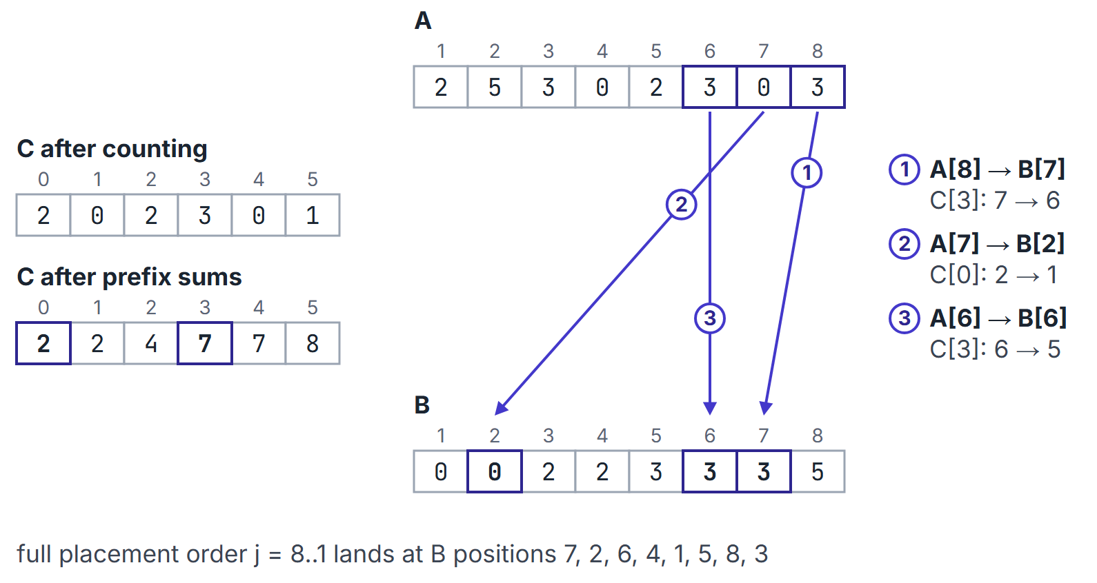
, , .
| 0 | 1 | 2 | 3 | 4 | 5 | |
|---|---|---|---|---|---|---|
| after counting | 2 | 0 | 2 | 3 | 0 | 1 |
| after prefix sums | 2 | 2 | 4 | 7 | 7 | 8 |
Placement from down: goes to ; to ; to ; to ; to ; to ; to ; to . Result .
Analysis
- Time : two loops over , two over . Linear when ; poor when (for example sorting 10 numbers below ).
- Space auxiliary (arrays and ): not in place.
- Best, average and worst cases are the same: it never compares keys.
- Stable; works for records with integer keys, not only for bare integers.
- Negative keys or keys in : shift by and use .
Radix sort
Purpose. Sort keys made of digits by sorting on one digit at a time, using a stable sort for each digit.
RADIX-SORT(A, d)
    for i <- 1 to d                     // digit 1 is the least significant
        use a stable sort to sort A on digit i
This is least significant digit (LSD) radix sort. It must start from the least significant digit, and the per-digit sort must be stable: after sorting on digit , keys that tie on digit stay ordered by digits from the earlier passes. By induction, after pass the keys are sorted on their last digits.
Worked example
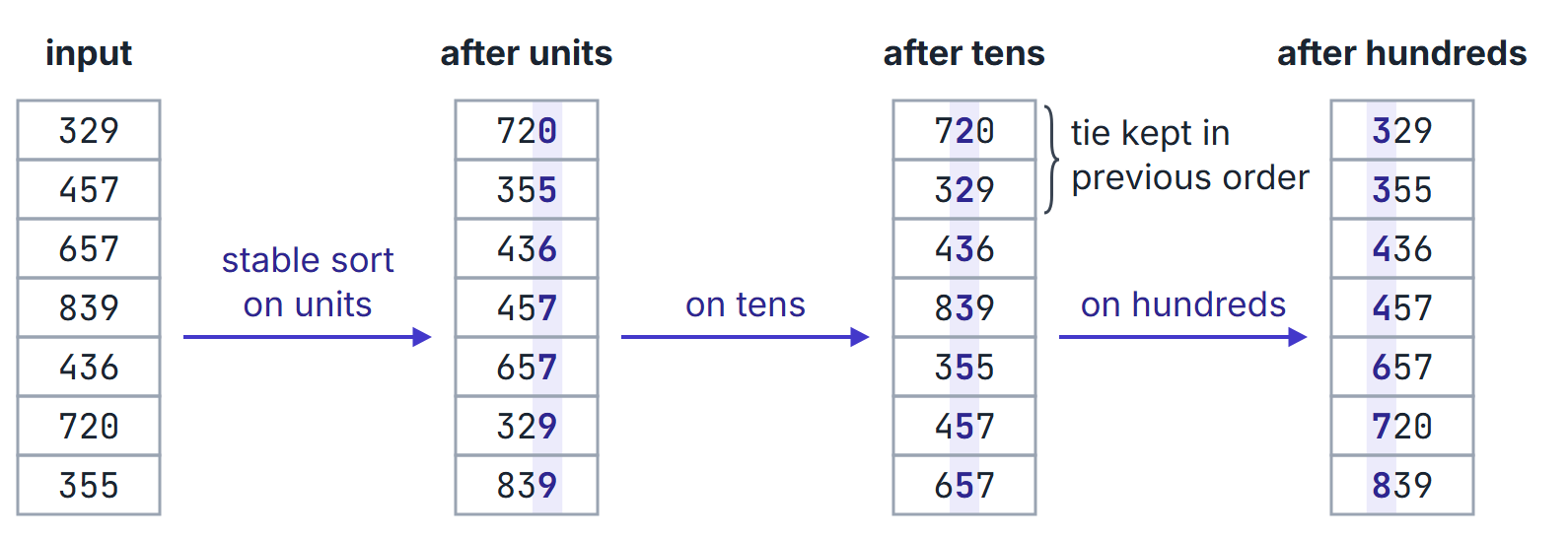
Seven 3-digit numbers, sorted with stable passes on units, tens and hundreds:
| Input | After units | After tens | After hundreds |
|---|---|---|---|
| 329 | 720 | 720 | 329 |
| 457 | 355 | 329 | 355 |
| 657 | 436 | 436 | 436 |
| 839 | 457 | 839 | 457 |
| 436 | 657 | 355 | 657 |
| 720 | 329 | 457 | 720 |
| 355 | 839 | 657 | 839 |
In the tens pass, 720 and 329 have tens digits 2 and 2; they stay in their units-pass order (720 before 329) because the pass is stable. In the final pass the hundreds digits decide.
Analysis
- With counting sort as the stable per-digit sort and digits in : each pass is , so the total is . Linear when is constant and .
- Choosing the digit size. For integer and keys of bits, split each key into digits of bits; then and the time is . Taking (for ) gives . Example: keys of bits with need 2 passes with .
- Space with counting sort; not in place.
- Stable (if every pass is stable).
- Most significant digit first works only with recursion into each bucket (MSD radix sort); running plain passes from the most significant digit gives a wrong result. On the worked example, stable passes on hundreds, then tens, then units end with 720 355 436 457 657 329 839: the last pass wins, so the list is ordered primarily by the units digit.
- For and a fixed integer , integers can be sorted in time: write them in base , using digits in .
Bucket sort
Purpose. Sort real numbers that are drawn independently and uniformly from .
BUCKET-SORT(A, n)
    create empty lists B[0..n-1]
    for i <- 1 to n
        insert A[i] into list B[floor(n * A[i])]
    for i <- 0 to n - 1
        sort list B[i] with insertion sort
    concatenate B[0], B[1], ..., B[n-1] in order
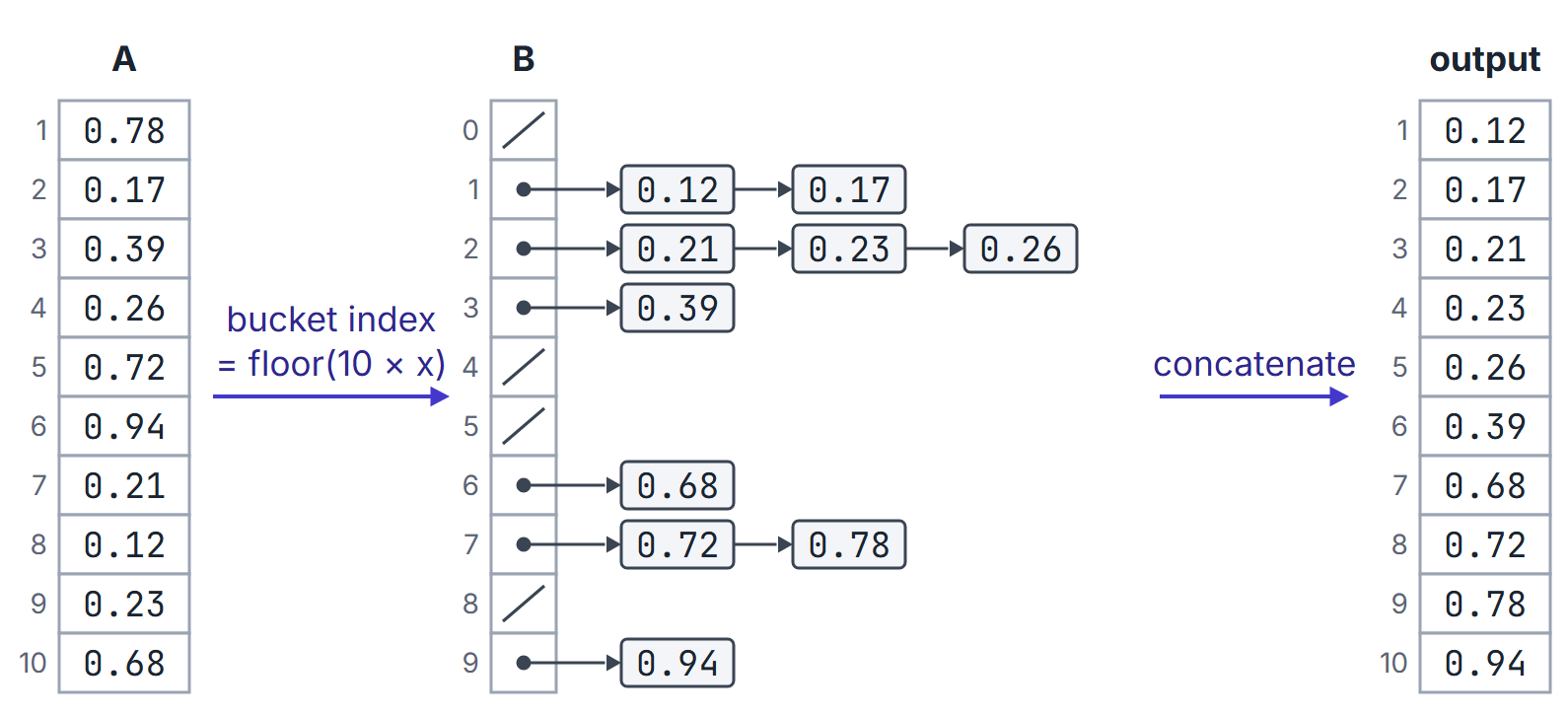
Example. , . Bucket : bucket 1 gets 0.17, 0.12; bucket 2 gets 0.26, 0.21, 0.23; bucket 3 gets 0.39; bucket 6 gets 0.68; bucket 7 gets 0.78, 0.72; bucket 9 gets 0.94; buckets 0, 4, 5 and 8 stay empty. After sorting each bucket and concatenating: 0.12 0.17 0.21 0.23 0.26 0.39 0.68 0.72 0.78 0.94.
Analysis
- Distribution and concatenation: .
- If is the size of bucket , insertion sort costs . Under the uniform assumption, , so the expected total is .
- Worst case : if all keys fall into one bucket, insertion sort runs on all . Using merge sort inside buckets lowers the worst case to .
- Space for the buckets. Stable if insertion into buckets appends and the bucket sort is stable.
- The linear bound holds more generally whenever the sum of the squares of the bucket sizes is linear in expectation; with a non-uniform but known distribution, choose bucket boundaries at its quantiles.
Comparison
| Property | Counting sort | Radix sort (LSD) | Bucket sort |
|---|---|---|---|
| Key assumption | integers | digits in | uniform on |
| Time | all cases | all cases | expected, worst |
| Auxiliary space | |||
| Stable | yes (right-to-left placement) | yes (needs stable passes) | yes, if bucket sort is stable |
| In place | no | no | no |
| Comparison-based | no | no | partly (inside buckets) |
Important properties and observations
- These algorithms do not contradict the lower bound: it applies only to algorithms that learn about keys by comparisons.
- Counting sort is the standard stable subroutine for radix sort. Replacing it by an unstable sort (for example, quicksort on each digit) breaks radix sort.
- "Linear" depends on the parameters: counting sort with is ; radix sort with digits and is ; in general its cost is .
- Counting sort can also count, for each value, how many keys are it: range-count queries in after preprocessing.
GATE examination perspective
- Counting sort traces. the count array after counting and after prefix sums, and the position each element lands in. Remember the right-to-left final loop.
- Radix sort traces. the list after a given pass; each pass must keep ties in their previous order.
- Complexity with parameters. express time in , , or and ; decide whether it is linear.
- Traps. radix sort needs a stable digit sort and must go from the least significant digit (the last pass decides the primary order); counting sort's final loop must run right to left when holds last positions; bucket sort's linear time is an expectation under the uniform assumption.
Summary
Sources
- T. H. Cormen, C. E. Leiserson, R. L. Rivest, C. Stein, Introduction to Algorithms, 3rd ed., MIT Press, 2009: Chapter 8, Sections 8.2 (counting sort), 8.3 (radix sort) and 8.4 (bucket sort and its expected-time analysis).