
Introduction
Chance is described with numbers: the number of heads in ten tosses, the number of probes in a hash table, the waiting time until a server responds. A random variable attaches a number to each outcome of an experiment, so that we can talk about its distribution, its average value (expectation) and its spread (variance). These three ideas are used throughout algorithm analysis (expected running time, expected number of collisions in hashing), performance modelling and statistics.
Prerequisites
- Probability Basics: sample spaces, events, independence.
- Integration: definite integrals, for continuous random variables.
Core concepts
Random variables
A random variable (RV) is a function from the sample space to . Example: toss three coins and let be the number of heads; the outcome gives . The event is the set of outcomes mapped to .
- is discrete if it takes finitely or countably many values.
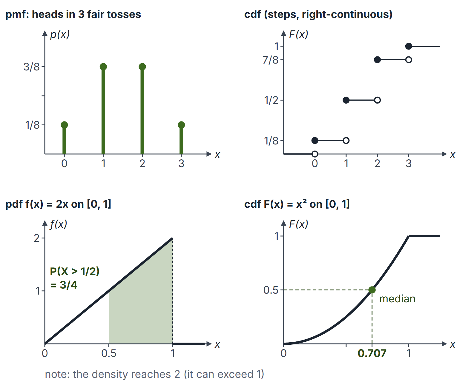
- is continuous if its probabilities are given by a density function, defined in the next table; then for every single value .
PMF, PDF and CDF
| Discrete RV | Continuous RV | |
|---|---|---|
| Described by | probability mass function (pmf) | probability density function (pdf) |
| Conditions | , | , |
| 0 | ||
| Value at a point | a probability, at most 1 | a density; can exceed 1 |
The cumulative distribution function (cdf) is defined for every RV as
Properties: is non-decreasing, right-continuous, as and as ; . For a discrete RV, is a step function jumping by at each value . For a continuous RV, is continuous and almost everywhere (and at every point where the chosen density is continuous). For a continuous RV, and give the same probabilities.
Expectation
The expected value (mean) is the probability-weighted average:
provided the sum or integral converges absolutely (otherwise does not exist).
Law of the unconscious statistician (LOTUS): for a function , or . There is no need to find the distribution of first.
Linearity of expectation: for any RVs and constants ,
whether or not and are independent. This is a key fact in probabilistic algorithm analysis.
Products: if and are independent. The converse is false.
Indicator variables. For an event , the indicator is 1 if occurs and 0 otherwise, so . Writing a count as a sum of indicators and using linearity avoids computing its distribution (Example 3).
Tail-sum formula. For an RV taking values in , .
Variance and standard deviation
The second form (the shortcut) follows by expanding the square and using linearity. Properties, for constants :
- , with equality if and only if is constant with probability 1.
- : shifting does not change spread; scaling by scales by .
- , where .
- If are independent (or merely uncorrelated), . Note the plus sign for the difference.
Variance convention. The variance of a random variable (a population quantity) is defined as the expectation , with no or divisor. The sample variance of observed data uses a divisor and is covered in Descriptive Statistics.
Joint distributions (brief)
For discrete , the joint pmf gives the marginals . and are independent if for all . When both variances are finite and positive, the correlation coefficient lies in . If either variable is constant, is undefined, not automatically zero. With finite positive variances, independence implies ; uncorrelated does not imply independent: if is uniform on and , then but is determined by .
Covariance and correlation rules
Every rule involving correlation below assumes finite, strictly positive variances for both variables.
For RVs and constants :
- , , and .
- Covariance is bilinear: and . Shifts drop out.
- For , : correlation has no units and ignores shifts and positive rescaling.
- if and only if with probability 1 for some , and then has the sign of .
- .
Conditional expectation. For discrete RVs, . The law of total expectation is the expectation form of total probability:
Inequalities
- Markov: if and , then .
- Chebyshev: for finite variance and , . If , taking , , gives . Thus at least lies strictly within standard deviations.
Worked examples
Example 1: a fair die
uniform on . . , so . For the sum of two independent dice: , . For : , .
Example 2: a continuous RV
for , and 0 otherwise. Check: . CDF: on . ; ; . . The median solves : .
Example 3: indicators (expected fixed points)
A random permutation of items. Let indicate that item is in place; . The number of fixed points has , for every , although the are dependent.
Example 4: hashing
keys hashed independently and uniformly into slots. Slot is empty with probability , so the expected number of empty slots is . With this is about , close to . The expected number of colliding pairs is .
Example 5: finding in a pmf
for . Then , so ; ; ; .
Example 6: a joint pmf table
| 0.2 | 0.1 | 0.3 | |
| 0.2 | 0.5 | 0.7 | |
| 0.4 | 0.6 | 1 |
, , and , so . As Bernoulli variables, and , so . and are dependent: . Finally , which matches the direct computation from the pmf of (values 0, 1, 2 with probabilities 0.2, 0.3, 0.5).
Example 7: law of total expectation
Roll a fair die, then toss a fair coin as many times as the die shows. Let be the die result, hence the number of coin tosses. Given , the expected number of heads is , so .
Example 8: expected inversions
In a random permutation of distinct keys, each of the pairs is out of order with probability . By indicators and linearity, the expected number of inversions is : 3 for , 4950/2 = 2475 for . This is the average number of adjacent swaps in bubble sort and adjacent-swap insertion sort; in the usual shift-based insertion sort it is the average number of rightward shifts.
Example 9: a function of a continuous RV
uniform on and . Use the cdf: for , , so , a density that is unbounded near 0 yet integrates to 1. By LOTUS, , which differs from by . The median of is : medians pass through increasing functions, means do not.
Important properties and observations
- , since the difference is the variance.
- and in general; only linear functions pass through .
- The mean minimises over constants ; the minimum value is .
- A pdf value is not a probability; only areas under are.
- For a non-negative continuous RV, .
GATE examination perspective
- Normalisation. Find the unknown constant in a pmf or pdf from total probability 1, then compute probabilities, mean or variance.
- Mean and variance computations. Use ; use .
- Linearity with indicators. Expected number of fixed points, empty bins, inversions, records; no independence needed.
- CDF questions. Probabilities from ; pdf as the derivative of the cdf; for a continuous CDF, a median solves . Generally a median satisfies and .
- Trap: adding variances of dependent RVs, or subtracting variances for .
- Trap: treating a density value larger than 1 as an error.
- Joint tables. Marginals, , covariance, correlation, and an independence check cell by cell (Example 6).
- Trap: concluding independence from ; one cell with proves dependence.
Summary
Sources
- S. Ross, A First Course in Probability, 8th ed., Pearson Prentice Hall, 2010, Chapters 4 (Random Variables) and 5 (Continuous Random Variables), Sections 7.2 (Expectation of Sums of Random Variables), 7.4 (Covariance, Variance of Sums, and Correlations) and 8.2 (Chebyshev's Inequality and the Weak Law of Large Numbers).