Discrete Distributions: Uniform, Binomial and Poisson

These distributions model the standard counting situations: picking uniformly from a finite set, counting successes in repeated independent trials, waiting for the first success, and counting rare events in a fixed interval. For each one you should know the pmf, the mean and variance, the situation it models, and how it connects to the others. The GATE syllabus names the uniform, binomial and Poisson distributions explicitly; the Bernoulli and geometric distributions are included because they are the building blocks.

A Bernoulli trial has two outcomes, success with probability $p$ and failure with probability $q = 1 - p$. A Bernoulli$(p)$ RV $X$ is the indicator of success:

$X$ is uniform on $\{a, a+1, \ldots, b\}$ if each of the $n = b - a + 1$ values has probability $1/n$. Then

For a fair die ($a = 1, b = 6$) this gives $3.5$ and $35/12$.

$X \sim \text{Bin}(n, p)$ counts successes in $n$ independent Bernoulli$(p)$ trials with the same $p$:

The pmf sums to 1 by the binomial theorem, $(p + q)^n = 1$. Writing $X$ as a sum of $n$ independent indicators gives

Shape: symmetric when $p = 1/2$, skewed right for $p < 1/2$ and left for $p > 1/2$. For $0<p<1$, the pmf increases while $k < (n + 1)p$ and decreases afterwards, so a mode is $\lfloor (n + 1)p \rfloor$; when $(n + 1)p$ is an integer, both $(n + 1)p$ and $(n + 1)p - 1$ are modes. At $p=0$ the unique mode is 0, and at $p=1$ it is $n$. Sums: if $X \sim \text{Bin}(n, p)$ and $Y \sim \text{Bin}(m, p)$ are independent (same $p$), then $X + Y \sim \text{Bin}(n + m, p)$.

When binomial does not apply. Drawing without replacement from a finite population makes trials dependent; the count then follows the hypergeometric distribution: $P(X = k) = \binom{K}{k}\binom{N - K}{n - k}/\binom{N}{n}$ for $K$ successes among $N$ items and $n$ draws. Its mean is still $nK/N$.

Geometric convention. $X$ is the number of the trial on which the first success occurs, so $X \in \{1, 2, 3, \ldots\}$. Then

Some books count the failures before the first success, $Y = X - 1 \in \{0, 1, \ldots\}$, with $E[Y] = q/p$ and the same variance. Read the question for which one is meant.

Geometric distributions here require $0<p\le1$. Memoryless property (for $0<p<1$, or only where the conditioning event has positive probability at $p=1$): $P(X > s + t \mid X > s) = P(X > t)$ for non-negative integers $s, t$. Having failed $s$ times tells you nothing about the remaining wait. The geometric is the only memoryless distribution on the positive integers.

$X \sim \text{Poisson}(\lambda)$, $\lambda > 0$, models the number of events in a fixed interval when events occur independently at a constant average rate:

The pmf sums to 1 because $\sum_k \lambda^k/k! = e^{\lambda}$. Useful facts:

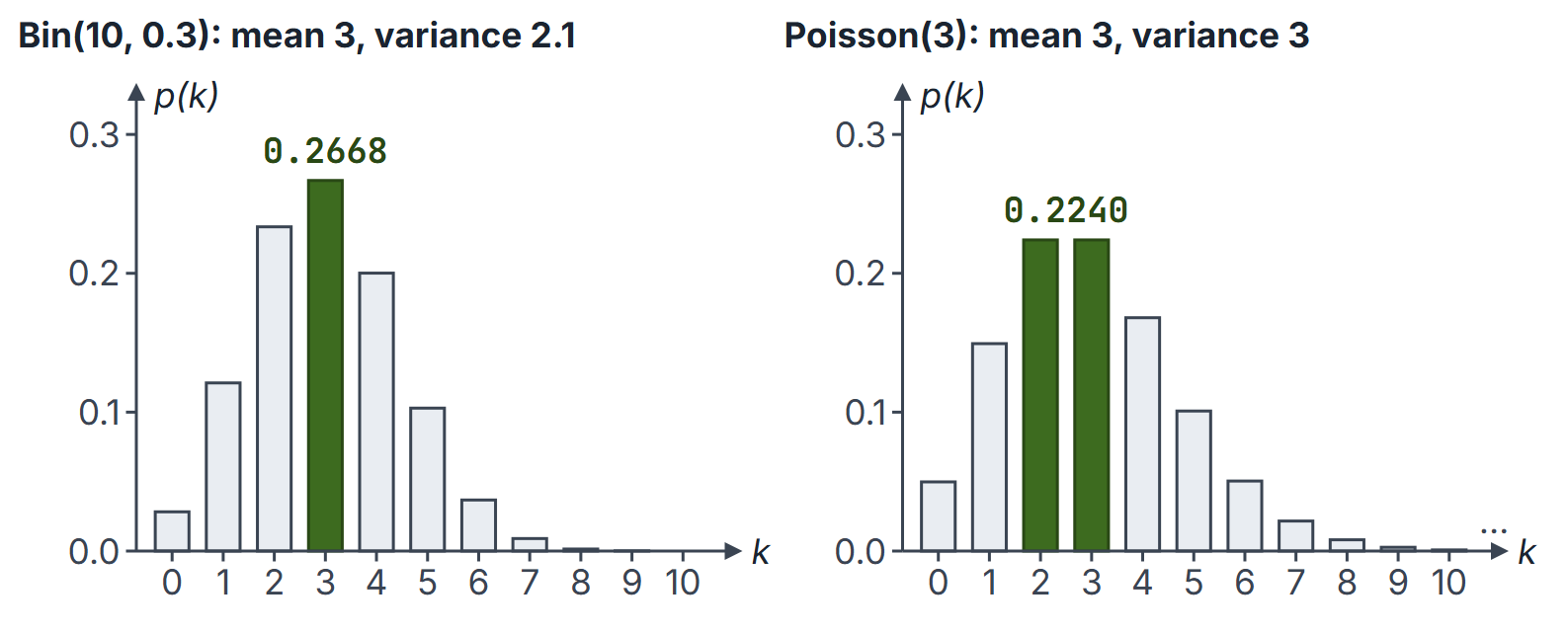
If $n$ is large, $p$ is small and $np = \lambda$ is moderate, then $\text{Bin}(n, p) \approx \text{Poisson}(np)$. Formally, for fixed $k$, $\binom{n}{k}p^k(1 - p)^{n-k} \to e^{-\lambda}\lambda^k/k!$ as $n \to \infty$ with $np = \lambda$ fixed. A common rule of thumb is $n \ge 20$ and $p \le 0.05$; it is a guideline, not a theorem.

Ten fair coins. $P(\text{exactly 4 heads}) = \binom{10}{4}/2^{10} = 210/1024 \approx 0.2051$. $P(\text{at least one head}) = 1 - 1/1024$. Mean 5, variance 2.5.

A binomial RV has mean 4 and variance 2.4. Then $q = 2.4/4 = 0.6$, $p = 0.4$ and $n = 4/0.4 = 10$. So $P(X = 0) = 0.6^{10} \approx 0.00605$. (If the given variance exceeded the mean, no binomial would fit, since $npq < np$.)

2% of chips are defective; a box holds 100. Exactly: $P(X = 0) = 0.98^{100} \approx 0.1326$. Poisson with $\lambda = 2$: $e^{-2} \approx 0.1353$. For $P(X \le 2)$: binomial $\approx 0.67669$, Poisson $5e^{-2} \approx 0.67668$. The approximation is excellent here.

Requests arrive at a server as a Poisson process with an average of 3 per minute. In one minute, $P(\text{none}) = e^{-3} \approx 0.0498$ and $P(\text{at least } 2) = 1 - e^{-3}(1 + 3) = 1 - 4e^{-3} \approx 0.8009$. In two minutes the count is Poisson$(6)$, so $P(\text{at least } 2) = 1 - 7e^{-6} \approx 0.9826$.

Roll a fair die until a 6 appears ($p = 1/6$). Expected rolls $= 6$; variance $= (5/6)/(1/36) = 30$. $P(\text{more than 4 rolls}) = (5/6)^4 \approx 0.4823$. By memorylessness, if the first 10 rolls had no six, the expected number of further rolls is still 6.

How many rolls until every face of a die has appeared? After $i$ distinct faces have been seen, the wait for a new one is geometric with $p = (6 - i)/6$, mean $6/(6 - i)$. By linearity,

In general $E[T] = n H_n \approx n \ln n$ for $n$ equally likely types.

Toss a fair coin until two consecutive heads appear; let $T$ be the number of tosses. Condition on the first tosses. Let $e_0$ be the expected number of further tosses from the start (or just after a tail) and $e_1$ the expected number just after one head:

Solving gives $e_1 = 4$ and $E[T] = e_0 = 6$. The same method for the pattern "head then tail" gives 4: after a head, a further head does not reset the progress. $T$ is not geometric, because successive attempts overlap.

Emails arrive as a Poisson process at 4 per hour, and each is spam with probability $1/4$, independently. The spam count in an hour is Poisson$(4 \times 1/4) =$ Poisson$(1)$ (thinning), so $P(\text{no spam in an hour}) = e^{-1} \approx 0.3679$. Conversely, given that exactly 5 emails arrived, the number of spam emails is $\text{Bin}(5, 1/4)$, so $P(\text{exactly 1 spam} \mid 5 \text{ emails}) = 5 \cdot \frac14 \cdot \left(\frac34\right)^4 = \frac{405}{1024} \approx 0.3955$.

Each attempt succeeds with probability $0.1$, independently. The smallest $n$ with $P(\text{at least one success}) = 1 - 0.9^n \ge 0.95$ satisfies $n \ge \ln 0.05/\ln 0.9 \approx 28.43$, so $n = 29$ ($1 - 0.9^{29} \approx 0.9529$, while $1 - 0.9^{28} \approx 0.9477$). Dividing by $\ln 0.9 < 0$ reverses the inequality.