Continuous Distributions: Uniform, Exponential and Normal

Continuous random variables describe measurements: a random point on an interval, the lifetime of a component, the time between requests, or exam marks spread around an average. Three continuous distributions cover the GATE syllabus. The uniform spreads probability evenly over an interval, the exponential models waiting times with no memory, and the normal describes sums of many small independent effects. For each, know the pdf, cdf, mean and variance, and the standard tricks: memorylessness for the exponential and standardisation for the normal.

$X \sim U(a, b)$, $a < b$, has constant density on $[a, b]$:

($F = 0$ left of $a$ and $F = 1$ right of $b$.) Probabilities are proportional to length: $P(c \le X \le d) = (d - c)/(b - a)$ for $a \le c \le d \le b$. Compare the discrete uniform variance $(n^2 - 1)/12$.

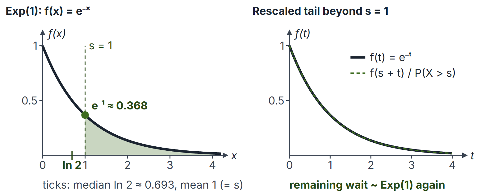
$X \sim \text{Exp}(\lambda)$ with rate $\lambda > 0$:

Rate versus mean. Some books parametrise by the mean $\theta = 1/\lambda$ and write $f(x) = \frac{1}{\theta}e^{-x/\theta}$. Always check whether a given number is a rate or a mean.

Memoryless property. For $s, t \ge 0$,

A component that has survived $s$ hours is "as good as new". The exponential is the only continuous distribution on $[0, \infty)$ with this property; it is the continuous analogue of the geometric.

Link with Poisson. If events occur as a Poisson process at rate $\lambda$ (the count in any interval of length $t$ is Poisson$(\lambda t)$, with independent counts in disjoint intervals), then the waiting time to the first event, and between events, is $\text{Exp}(\lambda)$. Indeed $P(T > t) = P(\text{no events in } [0, t]) = e^{-\lambda t}$.

Minimum of exponentials. If $X_1 \sim \text{Exp}(\lambda_1)$ and $X_2 \sim \text{Exp}(\lambda_2)$ are independent, then $\min(X_1, X_2) \sim \text{Exp}(\lambda_1 + \lambda_2)$ and $P(X_1 < X_2) = \lambda_1/(\lambda_1 + \lambda_2)$.

$X \sim N(\mu, \sigma^2)$ (second parameter is the variance) with $\sigma>0$ has density

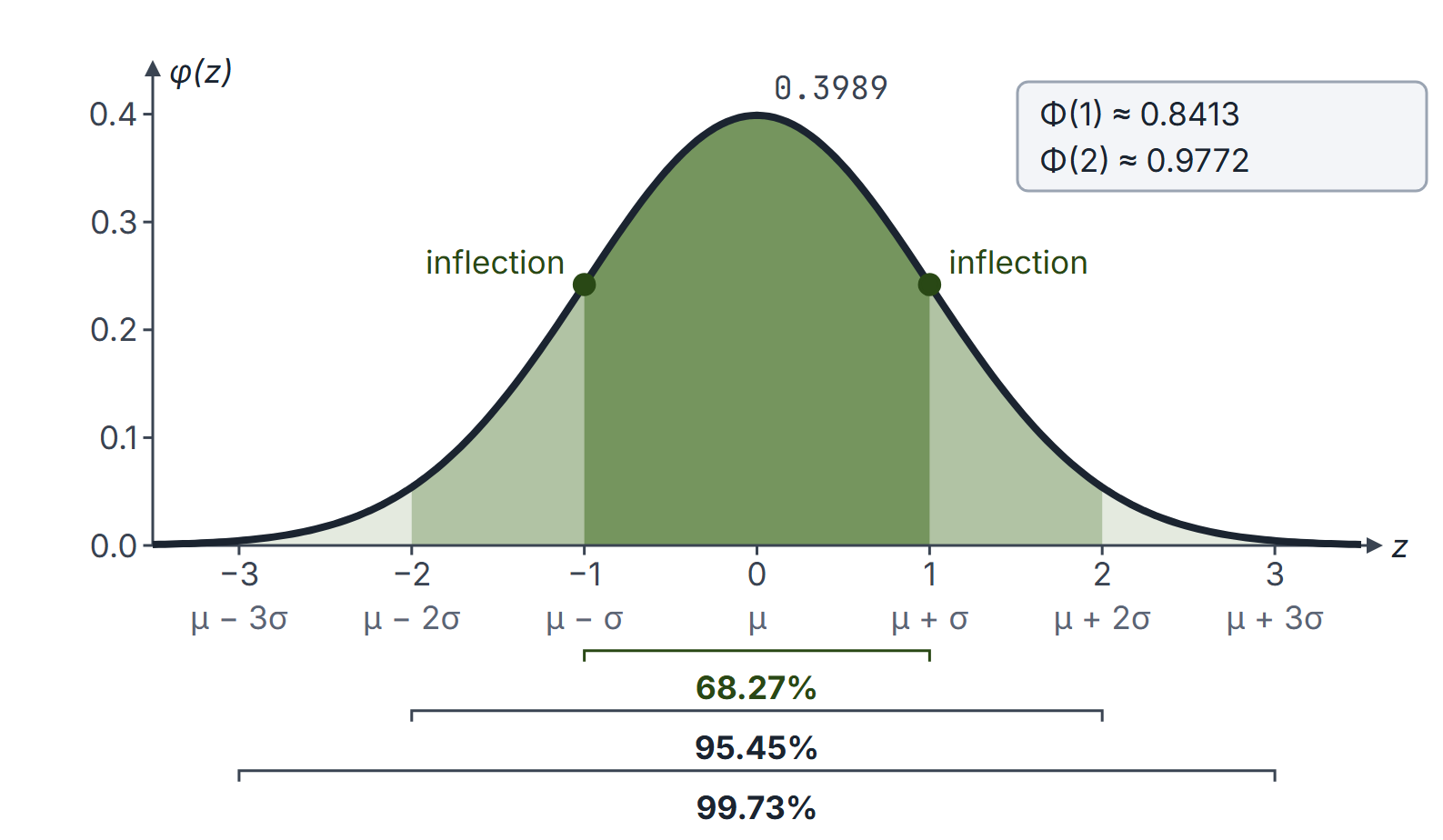
with $E[X] = \mu$ and $\operatorname{Var}(X) = \sigma^2$. The curve is bell-shaped and symmetric about $\mu$, so mean, median and mode are all $\mu$; its inflection points are at $\mu \pm \sigma$; the maximum height is $1/(\sigma\sqrt{2\pi})$.

Standardisation. $Z = (X - \mu)/\sigma \sim N(0, 1)$, the standard normal, with cdf $\Phi$. Hence

$\Phi$ has no closed form; a table, or the question, supplies values, or these standard ones are used: $\Phi(1) \approx 0.8413$, $\Phi(1.645) \approx 0.95$, $\Phi(1.96) \approx 0.975$, $\Phi(2) \approx 0.9772$, $\Phi(3) \approx 0.99865$.

Empirical rule. $P(|X - \mu| \le k\sigma) \approx 0.6827, 0.9545, 0.9973$ for $k = 1, 2, 3$. Compare Chebyshev's distribution-free bounds of at least $0, 0.75, 0.889$.

Linear combinations. If $X \sim N(\mu, \sigma^2)$, then $aX + b \sim N(a\mu + b, a^2\sigma^2)$ for $a \ne 0$. If $X_1, \ldots, X_n$ are independent normals, any linear combination $\sum c_i X_i$ is normal with mean $\sum c_i\mu_i$ and variance $\sum c_i^2\sigma_i^2>0$; if this sum is zero, the combination is constant rather than a nondegenerate normal.

Central limit theorem (informal). The sum of many independent, identically distributed RVs with finite variance is approximately normal. Consequently $\text{Bin}(n, p) \approx N(np, npq)$ when $np$ and $nq$ are both reasonably large (a common guide is at least 5 or 10). Use a continuity correction: $P(X \ge k) \approx P(Y \ge k - 0.5)$ for the normal approximation $Y$.

The exponential is right-skewed, so mode $<$ median $<$ mean, the order described in Descriptive Statistics. The median always solves $F(m) = 1/2$.

$X \sim U(0, 10)$. $P(3 < X < 7) = 4/10 = 0.4$; $E[X] = 5$; $\operatorname{Var}(X) = 100/12 = 25/3$.

Lifetimes are exponential with mean 1000 hours, so $\lambda = 1/1000$. $P(\text{lasts more than } 1000 \text{ h}) = e^{-1} \approx 0.3679$. Given it has lasted 500 hours, the probability it lasts beyond 1500 hours is again $e^{-1}$. The median lifetime is $1000 \ln 2 \approx 693$ hours, less than the mean because the distribution is right-skewed.

Marks are $N(60, 10^2)$. $P(X > 80) = 1 - \Phi(2) \approx 0.0228$. $P(50 < X < 70) = \Phi(1) - \Phi(-1) \approx 0.6827$.

$X \sim N(10, 9)$ and $Y \sim N(5, 16)$ are independent. Then $X - Y \sim N(5, 25)$ (variances add), so $P(X > Y) = P(Z > -1) = \Phi(1) \approx 0.8413$.

100 fair coin tosses; $P(\text{at least } 60 \text{ heads})$. Mean 50, standard deviation 5. With continuity correction: $P(Z \ge (59.5 - 50)/5) = 1 - \Phi(1.9) \approx 0.0287$. The exact binomial value is about $0.0284$.

Two independent servers finish jobs after $\text{Exp}(2)$ and $\text{Exp}(3)$ hours. The first completion time is $\text{Exp}(5)$, with mean $1/5$ hour = 12 minutes, and server 1 finishes first with probability $2/5$.

With marks $N(60, 10^2)$ as in Example 3, the cut-off $c$ for the top 10% satisfies $\Phi((c - 60)/10) = 0.90$. From tables $\Phi(1.2816) \approx 0.90$, so $c \approx 60 + 12.8 = 72.8$. Percentile questions run the standardisation backwards: $x = \mu + z\sigma$.

Contrast with the exponential. If $X \sim U(0, 4)$, then $P(X > 1) = 3/4$ but

Having already waited 1 unit makes a further wait of 1 unit less likely, because the support ends at 4. Only the exponential (continuous) and the geometric (discrete) forget the past.

$E[X] = \int_0^\infty x\lambda e^{-\lambda x}\,dx = \int_0^\infty e^{-\lambda x}\,dx = 1/\lambda$ (parts, or the tail formula $E[X] = \int_0^\infty P(X > x)\,dx$). Similarly $E[X^2] = 2/\lambda^2$, so $\operatorname{Var}(X) = 2/\lambda^2 - 1/\lambda^2 = 1/\lambda^2$.

$X, Y$ independent and uniform on $[0, 1]$. $P(\max(X, Y) \le t) = t^2$ and $P(\min(X, Y) > t) = (1 - t)^2$ for $0 \le t \le 1$, so by the tail formula $E[\max] = \int_0^1 (1 - t^2)\,dt = 2/3$ and $E[\min] = \int_0^1 (1 - t)^2\,dt = 1/3$. Since $|X - Y| = \max - \min$, $E|X - Y| = 1/3$. For $n$ independent uniforms, $E[\max] = n/(n + 1)$ and $E[\min] = 1/(n + 1)$.

Two servers work in parallel, each failing after an independent Exp$(\lambda)$ time, and the system fails when both have failed. $P(\text{system alive at } t) = 1 - (1 - e^{-\lambda t})^2$. By memorylessness, the first failure comes after a mean $1/(2\lambda)$ (minimum of two exponentials, rate $2\lambda$), and the survivor then lasts a fresh mean $1/\lambda$, so the expected system lifetime is $\frac{1}{2\lambda} + \frac{1}{\lambda} = \frac{3}{2\lambda}$. With $\lambda = 0.1$ per hour this is 15 hours, and the system is still alive at $t = 10$ with probability $1 - (1 - e^{-1})^2 \approx 0.6004$.