
Introduction
Descriptive statistics summarise a data set with a few numbers: where it is centred (mean, median, mode) and how spread out it is (range, variance, standard deviation). These are the sample counterparts of the expectation and variance of a random variable. The calculations are straightforward, but the divisor versus , the effect of shifting and scaling data, combining groups, and the order of mean, median and mode in a skewed distribution all need care.
Prerequisites
None within this subject. Basic arithmetic and summation notation suffice. Random Variables, Expectation and Variance gives the probabilistic view of the same ideas.
Core concepts
Throughout, the data are , and are the same values sorted.
Measures of central tendency
Arithmetic mean. . For values with frequencies , . Key facts:
- : deviations from the mean cancel.
- minimises over constants .
- Combined mean of groups with sizes and means : .
- The mean is sensitive to outliers.
Median. The middle value of the sorted data: if is odd, and the average if is even (the usual convention). The median minimises and is robust to outliers.
Mode. The most frequent value. A data set can have no mode (all values distinct, under the usual convention), one mode, or several (bimodal, multimodal).
Grouped data (class width , total frequency ):
where for the median is the lower boundary of the class containing the -th value, the cumulative frequency before it and its frequency; for the mode is the lower boundary of the modal class, its frequency and the frequencies of the classes before and after. These are interpolation formulas, not exact values.
Other means for positive data: geometric mean and harmonic mean . Always , with equality if and only if all values are equal. For two numbers, .
Measures of dispersion
- Range .
- Mean absolute deviation about the mean: .
- Quartiles and the interquartile range . Textbooks use slightly different rules for quartiles of small data sets, so check which rule the question uses before computing.
- Variance and standard deviation, in two versions:
Divisor convention. Sample formulas with divisor require . Use the divisor when the data are the whole population, and when the data are a sample used to estimate the population variance ( is then an unbiased estimator). Check whether the question's "variance" uses divisor or ; if the options contain both values, decide which the question means. The standard deviation is the square root: or .
Shortcut formula (population): . Equivalently, the variance is the mean of squares minus the square of the mean, mirroring .
Coefficient of variation: , often as a percentage, using or consistently. The quotient requires a nonzero mean. Interpreting CV as relative spread normally requires a positive-mean ratio-scale quantity with a meaningful zero; arbitrary shifted scales such as Celsius do not support that interpretation. Positive rescaling preserves CV; shifting generally does not.
Effect of shifting and scaling
If every value is transformed as :
| Statistic | New value |
|---|---|
| mean, median | |
| mode values, | ; if , all observations equal , the unique mode |
| quartiles, | |
| quartiles, | (order reverses) |
| quartiles, | every quantile equals |
| range, IQR, standard deviation, mean deviation | times the old value |
| variance | times the old value |
Adding a constant shifts location but leaves spread unchanged.
Combined variance (population form) of two groups with sizes , means , variances and combined mean , with :
Skewness: where mean, median and mode sit
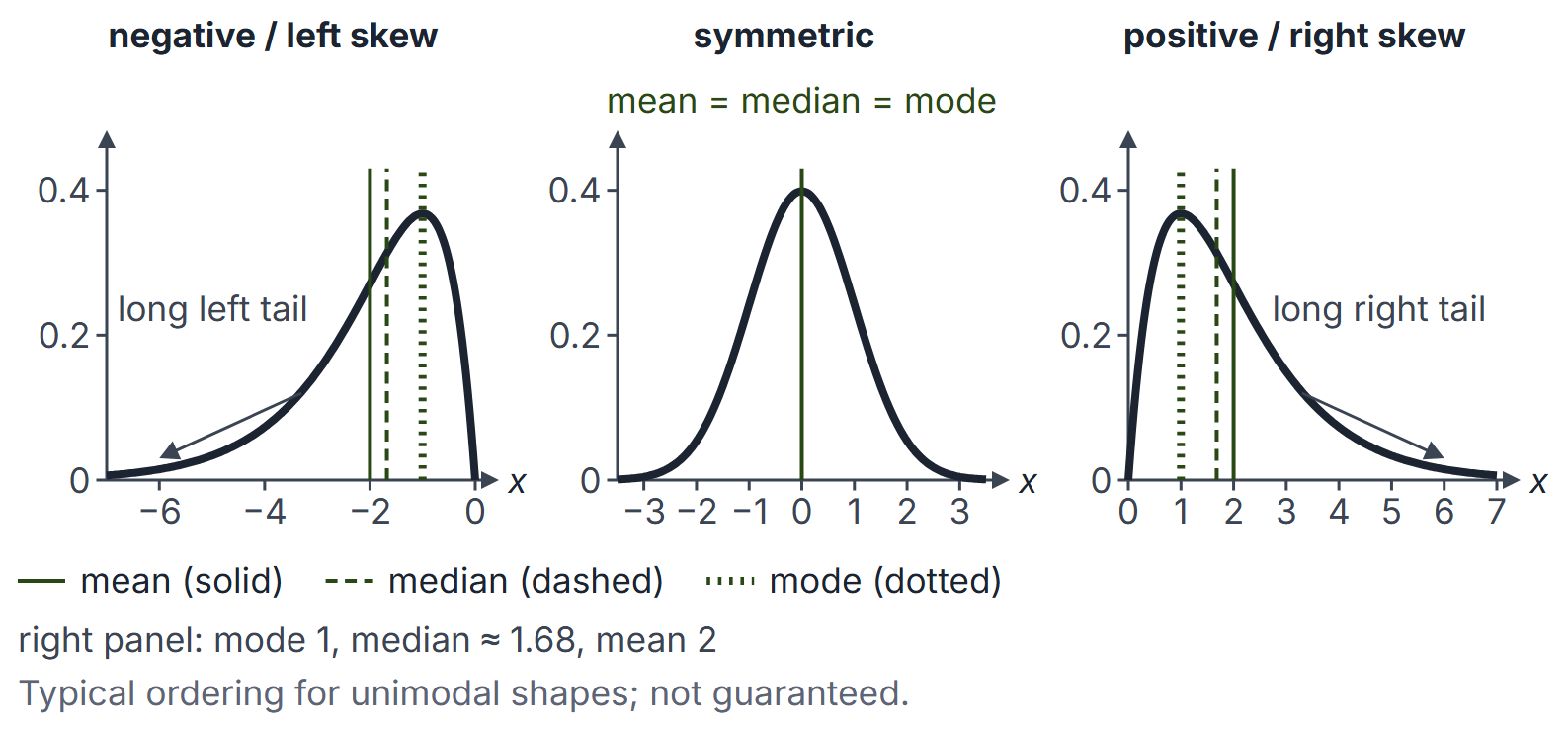
- Symmetric unimodal: mean = median = mode.
- Positively (right) skewed, long right tail: typically mode median mean. Incomes and waiting times look like this.
- Negatively (left) skewed: typically mean median mode.
These orderings are typical, not guaranteed; counterexamples exist for unusual shapes. Pearson's empirical relation holds approximately for moderately skewed unimodal data. It is not an identity. Pearson's coefficient of skewness is typically positive for ordinary right-skewed unimodal shapes; in unusual distributions its sign need not agree with moment skewness.
Paired data: covariance and correlation
For paired observations , , sample covariance requires . Pearson's additionally requires nonzero variation in both variables; it is undefined if either is constant. The formulas are
The divisor cancels in , so is the same whether or is used throughout. Always ; exactly when the points lie on a line with non-zero slope; is unchanged by shifting either variable and by multiplying it by a positive constant, and changes sign under a negative constant. measures linear association only: for on , although is a function of .
Worked examples
Example 1: a small data set
Data: (). Mean . Median . Mode . Squared deviations sum to , so the population variance is (), and the sample variance is (). Shortcut check: and . Range .
Example 2: combining groups
Group A: 30 students, mean 60, standard deviation 10. Group B: 20 students, mean 70, standard deviation 5. Combined mean ; , . Combined variance , standard deviation .
Example 3: change of units
Temperatures in Celsius have mean 20 and standard deviation 5. In Fahrenheit, : mean , standard deviation , variance .
Example 4: correcting an error
The mean of 10 observations is 15. One value, 12, was recorded as 21. The corrected total is , so the corrected mean is .
Example 5: grouped data
| Class | 0 to 10 | 10 to 20 | 20 to 30 | 30 to 40 |
|---|---|---|---|---|
| Frequency | 5 | 8 | 12 | 5 |
, ; cumulative frequencies are , so the median class is 20 to 30. Median . Modal class 20 to 30: Mode .
Example 6: three means
For and : AM , GM , HM . Check .
Example 7: correlation of paired data
Data . Means , . Deviations: ; . Then , , , and . The sample covariance is . Converting to other units () leaves unchanged.
Example 8: quick formulas
- The population standard deviation of two numbers is : for 4 and 10 it is 3.
- The first natural numbers have mean and population variance : for , mean 5.5 and variance .
- One outlier moves the mean but barely moves the median: for the mean is 22.8 and the median 4. Prefer the median for skewed data such as incomes.
Important properties and observations
- Standard deviation is zero if and only if all values are equal.
- Adding a value equal to the mean leaves the mean unchanged but decreases the population variance unless all values were already equal (the new point has zero deviation).
- For , increasing the largest observation leaves the conventional median unchanged, but changes the mean and spread. For , the median is the average of the two values, so increasing the maximum changes it too.
- Variance has squared units; standard deviation is in the units of the data.
GATE examination perspective
- Direct computation of mean, median, mode, variance or standard deviation of a small data set; watch for the divisor.
- Transformations. Effect of on each statistic.
- Combining groups and correcting errors with totals .
- Skewness ordering of mean, median and mode.
- Trap: mixing and between steps.
- Trap: forgetting to sort before taking the median.
- Correlation of paired data. Compute deviations, then ; check that .
- Trap: reading as "no relationship"; it rules out only a linear one.
Summary
Sources
- S. M. Ross, Introduction to Probability and Statistics for Engineers and Scientists, 4th ed., Elsevier Academic Press, 2009: Chapter 2 (Descriptive Statistics).
- E. Kreyszig, Advanced Engineering Mathematics, 10th ed., Wiley, 2011: Chapter 24 (Data Analysis. Probability Theory).