Introduction

The definite integral measures accumulated quantity: area under a curve, total probability, an average value. The fundamental theorem of calculus turns its computation into finding an antiderivative. The working tasks are evaluating a definite or improper integral (a symmetry property often makes this quick), differentiating an integral with variable limits, finding an area between curves, and making a trapezoidal or Simpson estimate.

Prerequisites

  • Limits: the definite integral is a limit of sums, and improper integrals are limits.
  • Continuity and Differentiability: derivatives of standard functions, the chain rule, continuity on a closed interval.

Core concepts

Antiderivatives

FF is an antiderivative of ff if F′=fF' = f. Any two differ by a constant, written ∫f(x) dx=F(x)+C\int f(x)\,dx = F(x) + C. Standard forms:

f(x)f(x)∫f(x) dx\int f(x)\,dx
xnx^n (n≠−1n \ne -1)xn+1/(n+1)x^{n+1}/(n+1)
1/x1/xln⁡∣x∣\ln\lvert x \rvert
eaxe^{ax}eax/ae^{ax}/a for a≠0a\ne0; for a=0a=0, xx (plus the integration constant)
sin⁡x\sin x, cos⁡x\cos x−cos⁡x-\cos x, sin⁡x\sin x
sec⁡2x\sec^2 xtan⁡x\tan x
1/(1+x2)1/(1 + x^2)arctan⁡x\arctan x
1/1−x21/\sqrt{1 - x^2}arcsin⁡x\arcsin x

The definite integral

Split [a,b][a, b] into nn pieces of width h=(b−a)/nh = (b - a)/n and pick a point xk∗x_k^* in each. The Riemann sum ∑f(xk∗)h\sum f(x_k^*)h adds rectangle areas. If these sums tend to the same limit for every choice as h→0h \to 0, that limit is ∫abf(x) dx\int_a^b f(x)\,dx. Every continuous function on [a,b][a, b] is integrable, and so is every bounded function with finitely many jumps.

Area counts with sign: parts of the graph below the axis contribute negatively. For the geometric area use ∫ab∣f(x)∣ dx\int_a^b |f(x)|\,dx.

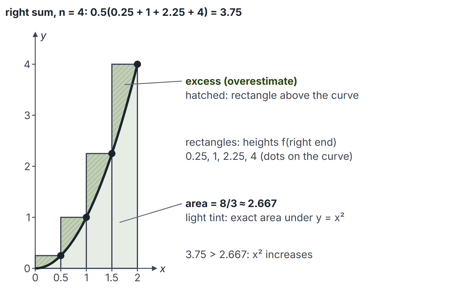
Right-endpoint Riemann sum for x^2 from 0 to 2
Figure 1. The area under y=x2y = x^2 on [0,2][0, 2] is 8/3≈2.6678/3 \approx 2.667. Four right-endpoint rectangles of width 0.5 give 3.753.75, an overestimate because x2x^2 increases. As the number of rectangles grows, the sum tends to 8/38/3.

Properties

  • Linearity: ∫ab(αf+βg)=α∫abf+β∫abg\int_a^b (\alpha f + \beta g) = \alpha\int_a^b f + \beta\int_a^b g.
  • Additivity: ∫abf+∫bcf=∫acf\int_a^b f + \int_b^c f = \int_a^c f; reversal: ∫baf=−∫abf\int_b^a f = -\int_a^b f.
  • Comparison: f≤gf \le g on [a,b][a, b]   ⟹  ∫abf≤∫abg\implies \int_a^b f \le \int_a^b g; also ∣∫abf∣≤∫ab∣f∣|\int_a^b f| \le \int_a^b |f|.
  • Mean value theorem for integrals: for continuous ff, ∫abf=f(c)(b−a)\int_a^b f = f(c)(b - a) for some c∈[a,b]c \in [a, b]. The average value of ff is 1b−a∫abf\frac{1}{b - a}\int_a^b f.

The fundamental theorem of calculus

Part 1. If ff is continuous on [a,b][a, b], then G(x)=∫axf(t) dtG(x) = \int_a^x f(t)\,dt is differentiable and G′(x)=f(x)G'(x) = f(x).

Part 2. If FF is any antiderivative of continuous ff, then ∫abf(x) dx=F(b)−F(a)\int_a^b f(x)\,dx = F(b) - F(a).

Variable limits (Leibniz rule). By Part 1 and the chain rule,

ddx∫u(x)v(x)f(t) dt=f(v(x)) v′(x)−f(u(x)) u′(x).\frac{d}{dx}\int_{u(x)}^{v(x)} f(t)\,dt = f(v(x))\,v'(x) - f(u(x))\,u'(x).

Techniques

  • Substitution: ∫abf(g(x))g′(x) dx=∫g(a)g(b)f(u) du\int_a^b f(g(x))g'(x)\,dx = \int_{g(a)}^{g(b)} f(u)\,du. Change the limits along with the variable.
  • By parts: ∫abu dv=[uv]ab−∫abv du\int_a^b u\,dv = [uv]_a^b - \int_a^b v\,du. Choose uu as the factor that simplifies when differentiated (a common order: logarithm, inverse trigonometric, algebraic, trigonometric, exponential).
  • Partial fractions for rational functions: 1(x+1)(x+2)=1x+1−1x+2\frac{1}{(x + 1)(x + 2)} = \frac{1}{x + 1} - \frac{1}{x + 2}.

Symmetry shortcuts

  • ff odd: ∫−aaf=0\int_{-a}^{a} f = 0. ff even: ∫−aaf=2∫0af\int_{-a}^{a} f = 2\int_0^a f.
  • Reflection: ∫abf(x) dx=∫abf(a+b−x) dx\int_a^b f(x)\,dx = \int_a^b f(a + b - x)\,dx. Adding the two forms often cancels the hard part (Example 5).
  • Period TT: ∫0nTf=n∫0Tf\int_0^{nT} f = n\int_0^T f.

Improper integrals

An integral with an infinite limit or an unbounded integrand is defined as a limit, for example ∫1∞f=lim⁡R→∞∫1Rf\int_1^\infty f = \lim_{R \to \infty}\int_1^R f. It converges if the limit is finite.

  • ∫1∞x−p dx\int_1^\infty x^{-p}\,dx converges if and only if p>1p > 1 (value 1/(p−1)1/(p - 1)).
  • ∫01x−p dx\int_0^1 x^{-p}\,dx converges if and only if p<1p < 1 (value 1/(1−p)1/(1 - p)).
  • ∫0∞xne−x dx=n!\int_0^\infty x^n e^{-x}\,dx = n! for integers n≥0n \ge 0 (the gamma integral); ∫−∞∞e−x2 dx=π\int_{-\infty}^{\infty} e^{-x^2}\,dx = \sqrt{\pi}.

Convergence trap. ∫−11dx/x2\int_{-1}^{1} dx/x^2 is improper (unbounded at 0) and diverges. Applying the antiderivative blindly gives −2-2, which is wrong.

Where the gamma and Gaussian integrals come from

Gamma integral. Let In=∫0∞xne−x dxI_n = \int_0^\infty x^n e^{-x}\,dx, so I0=1I_0 = 1. For n≥1n \ge 1, integrate by parts with u=xnu = x^n and dv=e−x dxdv = e^{-x}\,dx:

In=[−xne−x]0∞+n∫0∞xn−1e−x dx=0+nIn−1,I_n = \Big[-x^n e^{-x}\Big]_0^\infty + n\int_0^\infty x^{n-1} e^{-x}\,dx = 0 + n I_{n-1},

because xne−x→0x^n e^{-x} \to 0 as x→∞x \to \infty and the bracket is 0 at x=0x = 0. Hence In=n!I_n = n!. Substituting x=atx = at gives ∫0∞tne−at dt=n!/an+1\int_0^\infty t^n e^{-at}\,dt = n!/a^{n+1} for a>0a > 0, the source of the exponential moments E[Xn]=n!/λnE[X^n] = n!/\lambda^n in Continuous Distributions. The gamma function Γ(s)=∫0∞xs−1e−x dx\Gamma(s) = \int_0^\infty x^{s-1} e^{-x}\,dx extends the factorial: Γ(n+1)=n!\Gamma(n + 1) = n!.

Gaussian integral. Let G=∫−∞∞e−x2 dxG = \int_{-\infty}^{\infty} e^{-x^2}\,dx. It converges, since x2≥∣x∣−14x^2 \ge |x| - \frac14 gives e−x2≤e1/4e−∣x∣e^{-x^2} \le e^{1/4} e^{-|x|}. Square it, write the square as a double integral over the plane, and change to polar coordinates (x=rcos⁡θx = r\cos\theta, y=rsin⁡θy = r\sin\theta, area element r dr dθr\,dr\,d\theta):

G2=∫−∞∞∫−∞∞e−(x2+y2) dx dy=∫02π∫0∞e−r2 r dr dθ=2π⋅12=π,G^2 = \int_{-\infty}^{\infty}\int_{-\infty}^{\infty} e^{-(x^2 + y^2)}\,dx\,dy = \int_0^{2\pi}\int_0^\infty e^{-r^2}\,r\,dr\,d\theta = 2\pi \cdot \frac12 = \pi,

because ∫0∞re−r2 dr=[−12e−r2]0∞=12\int_0^\infty r e^{-r^2}\,dr = \big[-\tfrac12 e^{-r^2}\big]_0^\infty = \tfrac12. Since G>0G > 0, G=πG = \sqrt{\pi}. To make the limit step honest, note that the square [−R,R]2[-R, R]^2 lies between the discs of radius RR and R2R\sqrt{2}, so

π(1−e−R2)≤(∫−RRe−x2 dx)2≤π(1−e−2R2),\pi\big(1 - e^{-R^2}\big) \le \left(\int_{-R}^{R} e^{-x^2}\,dx\right)^2 \le \pi\big(1 - e^{-2R^2}\big),

and both bounds tend to π\pi. Consequences: ∫0∞e−x2 dx=π/2\int_0^\infty e^{-x^2}\,dx = \sqrt{\pi}/2 (even integrand); ∫−∞∞e−t2/2 dt=2π\int_{-\infty}^{\infty} e^{-t^2/2}\,dt = \sqrt{2\pi} (substitute x=t/2x = t/\sqrt{2}), the normalising constant of the normal density; and Γ(1/2)=∫0∞x−1/2e−x dx=π\Gamma(1/2) = \int_0^\infty x^{-1/2} e^{-x}\,dx = \sqrt{\pi} (substitute x=t2x = t^2).

Numerical integration

With nn strips of width hh and values y0,…,yny_0, \dots, y_n:

  • Trapezoidal rule: h2[y0+2(y1+⋯+yn−1)+yn]\frac h2[y_0+2(y_1+\cdots+y_{n-1})+y_n]. On a fixed interval [a,b][a,b], if f∈C2[a,b]f\in C^2[a,b], its absolute global error is at most (b−a)h2max⁡[a,b]∣f′′∣/12(b-a)h^2\max_{[a,b]}|f^{\prime\prime}|/12, hence O(h2)O(h^2); it is exact for straight lines.
  • Simpson's 1/3 rule (nn even): h3[y0+4(y1+y3+⋯ )+2(y2+y4+⋯ )+yn]\frac h3[y_0+4(y_1+y_3+\cdots)+2(y_2+y_4+\cdots)+y_n]. On fixed [a,b][a,b], if f∈C4[a,b]f\in C^4[a,b], the absolute global error is at most (b−a)h4max⁡[a,b]∣f(4)∣/180(b-a)h^4\max_{[a,b]}|f^{(4)}|/180, hence O(h4)O(h^4); it is exact for polynomials up to degree 3.

Worked examples

Example 1: the figure, as a limit

For x2x^2 on [0,2][0, 2] with nn right-endpoint rectangles, h=2/nh = 2/n and the sum is h3∑k=1nk2=8(n+1)(2n+1)6n2h^3\sum_{k=1}^{n} k^2 = \frac{8(n + 1)(2n + 1)}{6n^2}. For n=4n = 4 this is 3.75; as n→∞n \to \infty it tends to 16/6=8/316/6 = 8/3, matching [x3/3]02[x^3/3]_0^2.

Example 2: derivative of an integral

ddx∫0x2sin⁡t dt=2xsin⁡(x2)\frac{d}{dx}\int_0^{x^2}\sin t\,dt = 2x\sin(x^2). A limit that needs it: lim⁡x→01x3∫0xsin⁡(t2) dt\lim_{x \to 0}\frac{1}{x^3}\int_0^x \sin(t^2)\,dt is 0/00/0, and l'Hôpital gives lim⁡sin⁡(x2)3x2=13\lim \frac{\sin(x^2)}{3x^2} = \frac{1}{3}.

Example 3: substitution

∫012xex2 dx\int_0^1 2xe^{x^2}\,dx: with u=x2u = x^2, the limits become 0 and 1, so the value is ∫01eu du=e−1≈1.718\int_0^1 e^u\,du = e - 1 \approx 1.718.

Example 4: by parts

∫01xex dx=[xex]01−∫01ex dx=e−(e−1)=1\int_0^1 xe^x\,dx = [xe^x]_0^1 - \int_0^1 e^x\,dx = e - (e - 1) = 1. Similarly ∫1eln⁡x dx=[xln⁡x−x]1e=0−(−1)=1\int_1^e \ln x\,dx = [x\ln x - x]_1^e = 0 - (-1) = 1.

Example 5: reflection

I=∫0π/2sin⁡xsin⁡x+cos⁡x dxI = \int_0^{\pi/2}\frac{\sin x}{\sin x + \cos x}\,dx. Replacing xx by π/2−x\pi/2 - x swaps sine and cosine, so II also equals the integral of cos⁡xsin⁡x+cos⁡x\frac{\cos x}{\sin x + \cos x}. Adding, 2I=∫0π/21 dx=π/22I = \int_0^{\pi/2} 1\,dx = \pi/2, so I=π/4I = \pi/4.

Example 6: odd and even parts

∫−11x3cos⁡x dx=0\int_{-1}^{1} x^3\cos x\,dx = 0 (odd integrand). ∫−22∣x∣ dx=2∫02x dx=4\int_{-2}^{2} |x|\,dx = 2\int_0^2 x\,dx = 4. ∫−11(x3+x2) dx=0+2/3=2/3\int_{-1}^{1}(x^3 + x^2)\,dx = 0 + 2/3 = 2/3.

Example 7: improper integrals

∫1∞x−2 dx=1\int_1^\infty x^{-2}\,dx = 1; ∫1∞x−1 dx\int_1^\infty x^{-1}\,dx diverges (ln⁡R→∞\ln R \to \infty); ∫01x−1/2 dx=2\int_0^1 x^{-1/2}\,dx = 2. ∫0∞xe−x dx=1!=1\int_0^\infty xe^{-x}\,dx = 1! = 1: the mean of an exponential random variable with rate 1.

Example 8: area between curves

y=xy = x and y=x2y = x^2 meet at x=0x = 0 and x=1x = 1, with x≥x2x \ge x^2 between. Area =∫01(x−x2) dx=1/2−1/3=1/6= \int_0^1 (x - x^2)\,dx = 1/2 - 1/3 = 1/6.

Example 9: partial fractions

∫01dx(x+1)(x+2)=[ln⁡x+1x+2]01=ln⁡23−ln⁡12=ln⁡43≈0.2877\int_0^1\frac{dx}{(x + 1)(x + 2)} = \left[\ln\frac{x + 1}{x + 2}\right]_0^1 = \ln\frac{2}{3} - \ln\frac{1}{2} = \ln\frac{4}{3} \approx 0.2877.

Example 10: trapezoidal versus Simpson

∫01dx1+x=ln⁡2≈0.693147\int_0^1\frac{dx}{1 + x} = \ln 2 \approx 0.693147. With h=0.5h = 0.5, the values are 1,2/3,1/21, 2/3, 1/2.

  • Trapezoidal: 0.25(1+4/3+0.5)≈0.7083330.25(1 + 4/3 + 0.5) \approx 0.708333 (error about 0.0152).
  • Simpson: 0.53(1+8/3+0.5)≈0.694444\frac{0.5}{3}(1 + 8/3 + 0.5) \approx 0.694444 (error about 0.0013).

Example 11: average value

The average of sin⁡x\sin x on [0,π][0, \pi] is 1π∫0πsin⁡x dx=2π≈0.637\frac{1}{\pi}\int_0^\pi \sin x\,dx = \frac{2}{\pi} \approx 0.637.

Important properties and observations

  • The constant CC disappears in a definite integral; never carry it into F(b)−F(a)F(b) - F(a).
  • A definite integral is a number; the variable inside is a dummy (∫abf(x) dx=∫abf(t) dt\int_a^b f(x)\,dx = \int_a^b f(t)\,dt).
  • ∫axf\int_a^x f is continuous even when ff has jumps, and differentiable wherever ff is continuous.
  • Check for points where the integrand blows up inside the interval before applying the fundamental theorem.
  • For a density ff: ∫f=1\int f = 1, P(a≤X≤b)=∫abfP(a \le X \le b) = \int_a^b f, E[X]=∫xf(x) dxE[X] = \int xf(x)\,dx; see Random Variables.
  • Simpson's rule needs an even number of strips; the trapezoidal rule overestimates for convex functions (f′′>0f'' > 0), as in Example 10.

GATE examination perspective

  • Evaluate a definite integral, looking for symmetry (odd function, reflection) or integrating by parts.
  • Improper integrals: convergence of ∫x−p\int x^{-p}, gamma-type integrals, and integrals of densities.
  • Leibniz rule: derivative of an integral with variable limits, or a 0/00/0 limit containing an integral.
  • Areas between curves.
  • Numerical: one or two steps of the trapezoidal or Simpson's rule, or which rule is exact for a given polynomial.
  • Trap: integrating straight across a singularity such as 1/x21/x^2 on [−1,1][-1, 1].

Summary

Sources

  1. G. Strang, Calculus, 3rd ed., Wellesley-Cambridge Press, 2017, Sections 5.4 (Indefinite Integrals and Substitutions), 5.5 (The Definite Integral), 5.6 (Properties of the Integral and Average Value), 5.7 (The Fundamental Theorem and Its Applications), 5.8 (Numerical Integration), 7.1 (Integration by Parts), 7.4 (Partial Fractions), 7.5 (Improper Integrals) and 8.1 (Areas and Volumes by Slices). Free edition on MIT OpenCourseWare, (consulted 2026-11-11).

Next steps