
Introduction
Probability measures how likely an uncertain outcome is, on a scale from 0 to 1. Impossible events have probability 0 and the certain event has probability 1; in general these values mean almost never/almost surely, not necessarily an empty/full event. In computer science it is used to analyse randomised algorithms (expected running time of quicksort with a random pivot), hashing (collision probability), networks (packet loss, collision in shared media), reliability of systems, and machine learning. The topics set up the language: experiments, sample spaces, events, the axioms, and the rules that follow from them, including the difference between mutually exclusive and independent events. Conditional probability and random variables build directly on it.
Prerequisites
Core concepts
Experiment, sample space, events
- A random experiment is a procedure with a well-defined set of possible results whose actual result is uncertain (tossing a coin, rolling a die, measuring a response time).
- The sample space (also ) is the set of all possible outcomes. Tossing two coins: .
- An event is a subset of . It occurs if the outcome lies in it. is the impossible event, the certain event.
- Set operations give new events: (" or "), (" and "), ("not "), (" but not ").
- and are mutually exclusive (disjoint) if . Events are exhaustive if . Nonempty mutually exclusive and exhaustive events form a partition of .
The axioms of probability
A probability assigns to each event a number such that:
- for every event ;
- ;
- for pairwise mutually exclusive events (finite or countably infinite), .
Everything else is derived from these three axioms (Kolmogorov).
Consequences
| Rule | Statement |
|---|---|
| Complement | |
| Impossible event | |
| Monotonicity | |
| Range | |
| Addition rule | |
| Difference | |
| Exactly one of | |
| Three events | |
| Union bound (Boole) | |
| Bonferroni |
The three-event rule is inclusion-exclusion; the sums run over the three events and the three pairs.
Classical (equally likely) probability
If is finite and every outcome is equally likely,
The equally likely assumption must be justified by the set-up (fair coin, fair die, random selection). Sums of two dice are not equally likely: but . Choose the sample space so that its outcomes are equally likely (ordered pairs of dice), then count.
When outcomes are not equally likely, is the sum of the probabilities of the outcomes in .
Sampling with and without replacement
Drawing items from , of which are "special":
- Without replacement: (the hypergeometric probability).
- With replacement: draws are independent with success probability , so (binomial; see Discrete Distributions).
Independence
Events and are independent if
Intuitively, knowing that occurred does not change the probability of (made precise with conditional probability). Facts:
- If and are independent, so are and , and , and .
- and are independent of every event.
- Events are mutually independent if for every subset of indices with . Pairwise independence (only ) is weaker.
- For mutually independent events, .
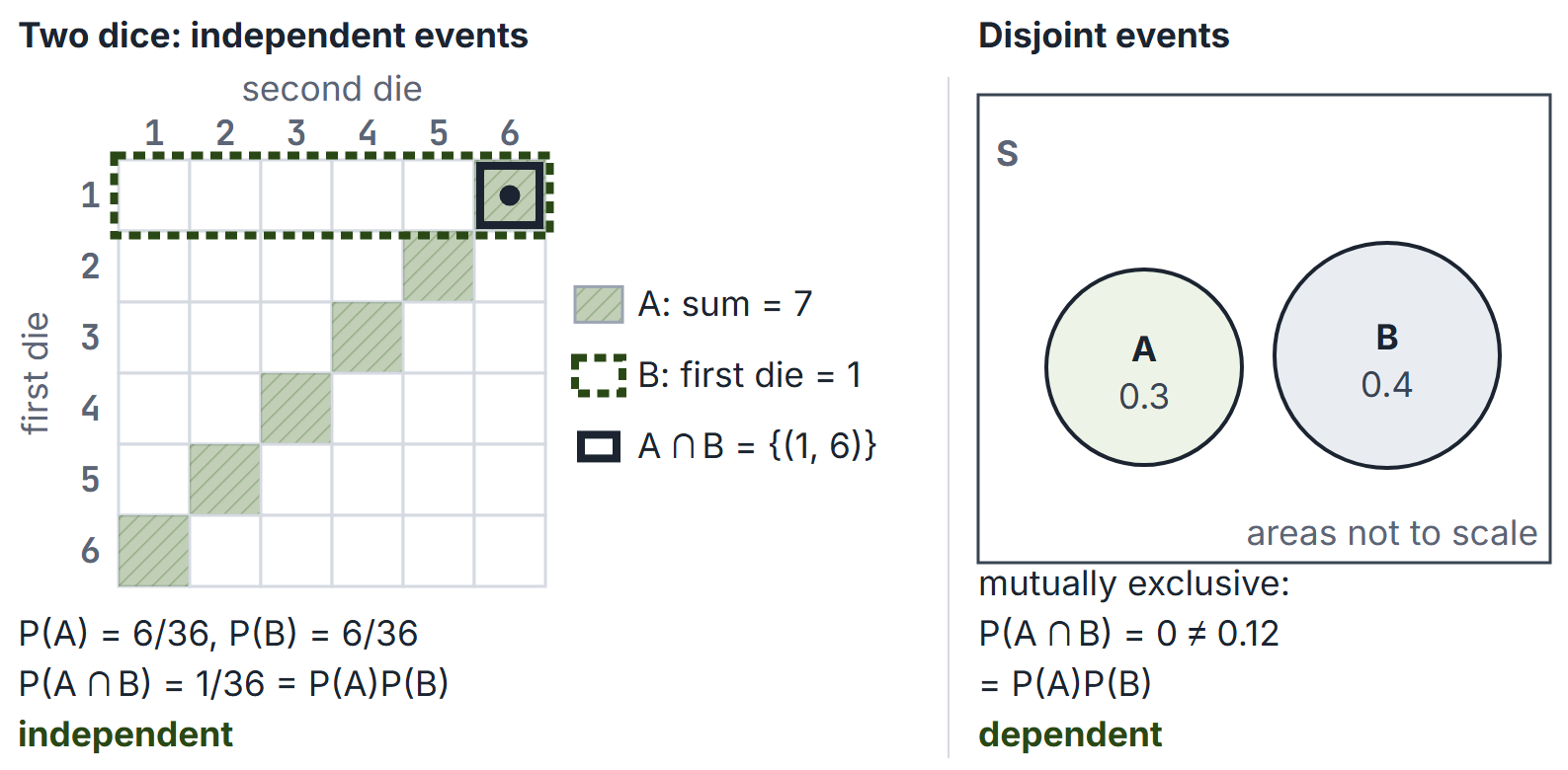
Mutually exclusive versus independent
These are different ideas; keep them apart.
| Mutually exclusive | Independent | |
|---|---|---|
| Definition | ||
| Depends on the probabilities? | No (a set property) | Yes |
| Can both hold? | Only if or | Only if or |
If and and are mutually exclusive, then : such events are dependent (if one happens, the other cannot).
Geometric probability
When an outcome is a point chosen uniformly from a region (an interval, a square), probability is a ratio of lengths or areas:
For two independent numbers , each uniform on , the pair is uniform on the unit square, so every event about and is a region of that square and its probability is the region's area. Points and lines have area 0, so and it does not matter whether an inequality is strict.
Worked examples
Example 1: two dice
Two fair dice. = "sum is 7", = "first die is 1", = "sum is 8". , , : independent. , (the second die would need 7): and are mutually exclusive, hence dependent.
Example 2: at least one
A system has 4 independent components, each failing with probability 0.1 during a day. .
Example 3: birthday problem
people, birthdays independent and uniform over 365 days (ignore leap years). . For , , just above . The same calculation bounds hash collisions: inserting keys into slots gives a collision with probability about .
Example 4: drawing cards
Two cards drawn without replacement from a standard 52-card deck. . With replacement: .
Example 5: pairwise but not mutually independent
Toss two fair coins. = "first is H", = "second is H", = "the two coins differ". Each has probability , and each pair intersects in one outcome of probability : pairwise independent. But , so : not mutually independent.
Example 6: addition rule
, , . Then , so are independent, and .
Example 7: meeting problem
Two friends arrive independently at uniformly random times between 5:00 and 6:00, and each waits 15 minutes for the other. Measure time in hours after 5:00, so are uniform on and they meet if . The complement is two corner triangles of the unit square with legs , of total area . So . With a waiting time (as a fraction of the window), . In the same square, (a half-square triangle).
Example 8: divisibility by inclusion-exclusion
A number is drawn uniformly from . Let be "divisible by "; the count of multiples of is . Then , , , , , , , and
The events are not independent here: . Always test independence by . For divisibility events with pairwise coprime divisors, a uniform consecutive-integer range whose length is divisible by their product is a sufficient, not necessary, shortcut for independence.
Example 9: taking turns
and toss a fair coin alternately, first, and the first head wins. wins on toss 1, 3, 5, and so on:
The game ends with probability 1, so . In general, independent trials with common success probability , and , give first-player win probability . For a die and “first six wins”, this is . At , both win probabilities are zero and nontermination has probability one.
Example 10: matching letters and envelopes
letters go into addressed envelopes at random. Let be "letter is in its own envelope". Any of these events occur together with probability , and there are such groups, so inclusion-exclusion gives
For : (9 of the 24 permutations are derangements), so at least one letter is correct with probability . The limit is reached quickly: already for the value is .
Important properties and observations
- Probabilities of a partition add to 1; this is the quickest consistency check on an answer.
- "At least one" is almost always computed as 1 minus "none".
- Independence is a property of the probability assignment, not of the events as sets; it cannot be read off a Venn diagram.
- Zero probability does not mean impossible for continuous outcomes (any single exact value of a continuous measurement has probability 0).
- always, with equality if and only if .
- Identical objects. Outcomes must be equally likely before counting. Put 2 identical balls into 2 boxes, each ball independently choosing either box with probability 1/2: the patterns , , have probabilities , not each. Label the objects, count, then forget the labels.
- The triple product alone is not enough. With 8 equally likely outcomes, , , satisfy , yet . Mutual independence of three events needs all four product equations.
GATE examination perspective
- Counting-based probability. Build an equally likely sample space (ordered outcomes, labelled objects), then count favourable outcomes.
- Union and complement. Inclusion-exclusion for two or three events; complements for "at least one".
- Independence checks. Compare with ; check all subsets for mutual independence.
- Trap: treating mutually exclusive events as independent, or the reverse.
- Trap: using on a sample space whose outcomes are not equally likely (sums of dice, numbers of heads).
- Geometric probability. Two uniform numbers on : draw the unit square and compute areas (meeting problems, ).
- Alternating turns and matching. A geometric series for "first to succeed wins"; inclusion-exclusion for "nobody gets their own".
- Trap: counting patterns of identical objects as if they were equally likely.
Summary
Sources
- S. Ross, A First Course in Probability, 8th ed., Pearson Prentice Hall, 2010: Chapter 2 (Axioms of Probability) and Section 3.4 (Independent Events).