Conditional Probability and Bayes Theorem

New information changes probabilities. Knowing that a test came back positive, that a packet arrived late, or that the first card drawn was an ace, we should update how likely the other events are. Conditional probability is the rule for that update. Two theorems follow from it: the law of total probability (compute a probability by splitting into cases) and Bayes theorem (reverse the direction of conditioning: from "probability of the evidence given the cause" to "probability of the cause given the evidence"). Bayes theorem underlies spam filters, diagnostic reasoning and naive Bayes classifiers.

For events $A$ and $B$ with $P(B) > 0$, the conditional probability of $A$ given $B$ is

Knowing $B$ occurred shrinks the sample space to $B$; $P(A \mid B)$ is the share of $B$ that also lies in $A$. With equally likely outcomes, $P(A \mid B) = |A \cap B| / |B|$. $P(A \mid B)$ is undefined when $P(B) = 0$.

For fixed $B$, $P(\cdot \mid B)$ is itself a probability: it satisfies the axioms, so $P(A^c \mid B) = 1 - P(A \mid B)$ and $P(A_1 \cup A_2 \mid B) = P(A_1 \mid B) + P(A_2 \mid B) - P(A_1 \cap A_2 \mid B)$. But in general $P(A \mid B^c) \ne 1 - P(A \mid B)$.

provided the conditioning events have positive probability. This is the rule for sequential experiments such as drawing without replacement.

For $P(B) > 0$: $A$ and $B$ are independent if and only if $P(A \mid B) = P(A)$. So independence means "learning $B$ does not change the probability of $A$".

$A$ and $B$ are conditionally independent given $C$ if $P(A \cap B \mid C) = P(A \mid C)\,P(B \mid C)$. Conditional independence and independence do not imply each other.

Let $B_1, \ldots, B_n$ be a partition of $S$ (mutually exclusive, exhaustive) with every $P(B_i) > 0$. Then for any event $A$:

The simplest case uses $B$ and $B^c$: $P(A) = P(A \mid B)P(B) + P(A \mid B^c)P(B^c)$.

With the same partition and $P(A) > 0$:

Vocabulary: $P(B_j)$ is the prior, $P(A \mid B_j)$ the likelihood, $P(B_j \mid A)$ the posterior, and the denominator is $P(A)$ by total probability. The posteriors over the partition add to 1.

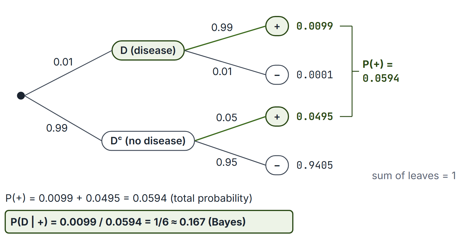
Probability tree method. Draw a branch for each $B_i$ labelled $P(B_i)$, then sub-branches for $A$ and $A^c$ labelled with conditional probabilities. Multiply along a path for the joint probability; add paths ending in $A$ for $P(A)$; divide one path by that sum for Bayes.

Confusing the two is the prosecutor's fallacy. They are related by Bayes: $P(B \mid A) = P(A \mid B)\,P(B)/P(A)$. They are equal only when $P(A) = P(B)$ (or $P(A \cap B) = 0$).

A disease affects 1% of a population. A test detects it in 99% of patients who have it (sensitivity), and gives a false positive for 5% of people who do not. A random person tests positive. What is the probability they have the disease?

Despite a 99% sensitive test, a positive result means only about a 1 in 6 chance of disease, because healthy people vastly outnumber sick ones. A second independent positive test (conditionally independent given the disease status) raises it to $\dfrac{0.99^2 \times 0.01}{0.99^2 \times 0.01 + 0.05^2 \times 0.99} = \dfrac{0.009801}{0.012276} \approx 0.798$.

Machines $M_1, M_2, M_3$ make 50%, 30% and 20% of a factory's items, with defect rates 1%, 2% and 3%.

A random item is defective. $P(M_3 \mid D) = 0.006/0.017 = 6/17 \approx 0.353$; similarly $P(M_1 \mid D) = 5/17$, $P(M_2 \mid D) = 6/17$. The three posteriors add to 1.

An urn has 5 red and 3 blue balls. Two are drawn without replacement.

A family has two children, each independently a boy or girl with probability $1/2$. Given that at least one is a boy, the probability that both are boys is $\dfrac{1/4}{3/4} = \dfrac{1}{3}$, not $1/2$. Given that the elder is a boy, it is $1/2$. The sample spaces differ: $\{BB, BG, GB\}$ versus $\{BB, BG\}$.

A prize is behind one of three doors. You pick door 1. The host, who knows where the prize is and always opens an unpicked door without the prize (choosing at random when he has a choice), opens door 3. Switching to door 2 wins with probability $2/3$: $P(\text{prize at 2} \mid \text{host opens 3}) = \dfrac{1 \cdot \frac13}{\frac12 \cdot \frac13 + 1 \cdot \frac13 + 0 \cdot \frac13} = \dfrac{2}{3}$. The answer depends on the stated host behaviour.

A transmitter sends 0 with probability 0.6 and 1 with probability 0.4. The channel flips a 0 into a 1 with probability 0.1, and a 1 into a 0 with probability 0.2.

Similarly $P(\text{receive } 0) = 0.62$ and $P(\text{sent } 0 \mid \text{receive } 0) = 0.54/0.62 = 27/31 \approx 0.871$. The probability of a correct decision when the receiver outputs whatever arrives is $0.54 + 0.32 = 0.86$.

Urn I has 3 white and 2 black balls; urn II has 4 white and 4 black. One ball is moved at random from urn I to urn II, then a ball is drawn from urn II. Split on the moved ball:

Given that the ball drawn is white, the moved ball was white with probability $\dfrac{15/45}{23/45} = \dfrac{15}{23} \approx 0.652$, up from the prior $3/5$.

A box holds one fair coin and one two-headed coin. A coin is picked at random and tossed twice. Given the coin, the tosses are independent. Unconditionally, $P(H_1) = P(H_2) = \frac12 \cdot \frac12 + \frac12 \cdot 1 = \frac34$, but

so the tosses are dependent: a first head is evidence for the two-headed coin. After two heads, $P(\text{two-headed} \mid H_1 \cap H_2) = \dfrac{1/2}{5/8} = \dfrac45$, and the next toss is a head with probability $\frac45 \cdot 1 + \frac15 \cdot \frac12 = \frac{9}{10}$.

Two fair dice. "At least one six" has 11 of the 36 outcomes, so $P(\text{both six} \mid \text{at least one six}) = 1/11$ and $P(\text{sum } 7 \mid \text{at least one six}) = 2/11$ (outcomes $(1, 6)$ and $(6, 1)$). Conditioning on "the first die is a six" instead gives $1/6$ for both. As in Example 4, the wording of the condition changes the reduced sample space.