Microprogrammed Control Unit: short notes (Computer Organization & Architecture)

Revision mode

Introduction

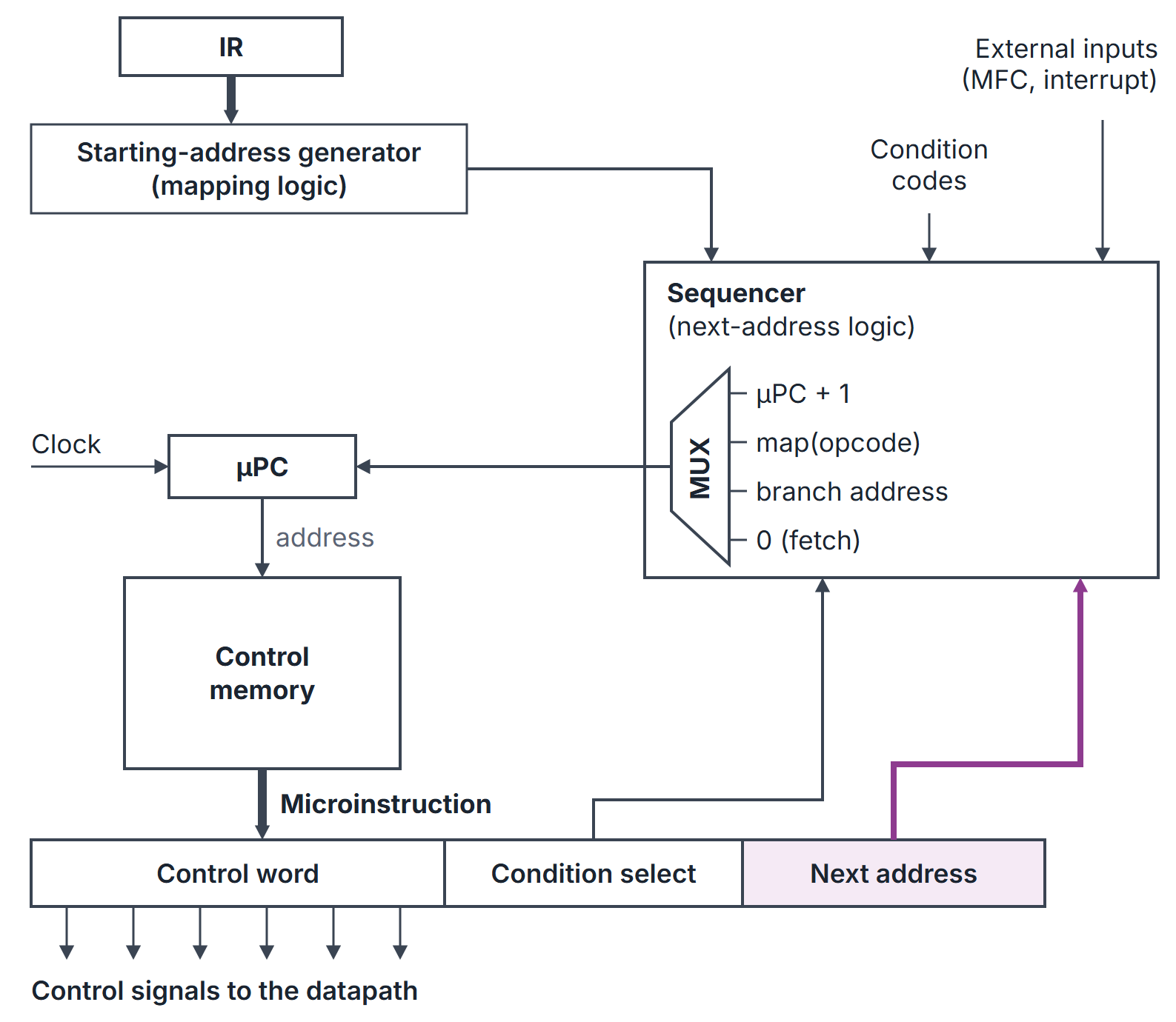
A microprogrammed control unit stores the control signals for every step of every instruction as words in a control memory (control store). Each word is a microinstruction; the sequence of microinstructions that carries out one machine instruction is its microroutine, and the whole contents of the control memory is the microprogram. A micro-program counter ( $\mu$ PC) steps through the control memory, and each microinstruction read out drives the datapath for one clock cycle.

GATE asks you to compute the width of a microinstruction and the size of the control memory, to compare horizontal and vertical formats, to size the fields of an encoded format, to work out the next-address and condition-select fields, and to compare microprogrammed with hardwired control. The control steps being stored come from CPU Datapath and Instruction Cycle.

Prerequisites

CPU Datapath and Instruction Cycle: control steps and the signals active in each step.

Core concepts

Terms

Term	Meaning
Control word (CW)	The set of control signal values for one step, as a bit string
Microinstruction	A CW plus any sequencing information (condition select, next address)
Control memory (CM)	Memory, usually ROM, holding the microprogram
$\mu$ PC or control address register (CAR)	Address of the next microinstruction
Starting-address generator (mapping logic)	Turns the opcode in IR into the address of its microroutine
Sequencer	Logic that chooses the next $\mu$ PC value

Sequencing the microprogram

After each microinstruction the $\mu$ PC is loaded with one of:

$\mu$ PC + 1, the next word (the common case);
the starting address of a microroutine, from the mapping logic, after the fetch microroutine has loaded IR;
a branch address, unconditionally or if a selected condition (a flag, MFC, an interrupt request) holds;
the fetch address (usually 0) at the end of each microroutine.

Two common ways to supply branch addresses:

Next-address field: every microinstruction carries the address of its successor (and a condition-select field picks which flag may modify it). There is no incrementer, but every word is wider.
Incrementer with branch microinstructions: only branching microinstructions carry an address; others fall through to $\mu$ PC + 1. Wide-branch addressing ORs bits of the opcode or of a flag into the low bits of the branch address so one microinstruction can branch many ways.

Horizontal and vertical microinstructions

Format	Encoding	Width	Parallelism	Decoding
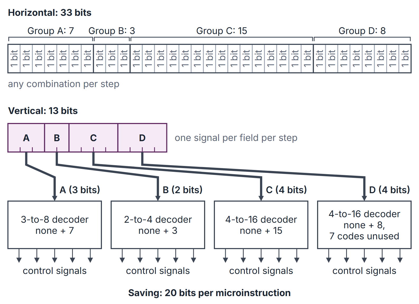
Horizontal	One bit per control signal	Widest (number of signals)	Any combination of signals in one step	None
Vertical	Signals grouped into encoded fields	Narrow	Only one signal per field per step	A decoder per field

A field groups signals that are never active in the same step (mutually exclusive, such as the sources that drive one bus). A field of $n$ signals needs $\lceil \lg(n+1) \rceil$ bits if a "no signal" code is needed, or $\lceil \lg n \rceil$ if exactly one is always active. Formats in between (a few fields, some single bits) are common and are still called vertical or, more precisely, field-encoded.

Microprogrammed against hardwired

Microprogrammed control is slower, because each step includes a control memory read, but it is regular, easy to modify or extend (new instructions mean new microroutines) and can emulate another instruction set by loading a different microprogram. Hardwired control is faster and suits simple, regular instruction sets; see Hardwired Control Unit.

How it works

Microprogrammed control unit: mapping logic, micro-PC, control memory and sequencer — Figure 1. Microprogrammed control: the starting-address generator maps the opcode in IR to a microroutine address; the $\mu$ PC, advanced by the sequencer using the clock, condition codes and external inputs, addresses the control memory, whose output word drives the control signals.

A small microprogram

Using the single-bus sequences of CPU Datapath and Instruction Cycle:

Address	Microinstruction (signals)	Next
0	PC $_{out}$ , MAR $_{in}$ , Read, Select4, Add, Z $_{in}$	1
1	Z $_{out}$ , PC $_{in}$ , Y $_{in}$ , WMFC	2
2	MDR $_{out}$ , IR $_{in}$	map(opcode)
10	R2 $_{out}$ , Y $_{in}$	11
11	R3 $_{out}$ , SelectY, Add, Z $_{in}$	12
12	Z $_{out}$ , R1 $_{in}$ , End	0
20	Offset $_{out}$ , SelectY, Add, Z $_{in}$	if $N = 0$ then 0 else 21
21	Z $_{out}$ , PC $_{in}$ , End	0

Here map(ADD R1, R2, R3) $= 10$ and map(BRN) $= 20$ . ADD takes 6 microinstructions (addresses 0, 1, 2, 10, 11, 12); BRN takes 4 when not taken and 5 when taken, the same step counts as the hardwired design.

Horizontal and vertical microinstruction formats for 33 control signals — Figure 2. The same 33 control signals as a 33-bit horizontal microinstruction and as a 13-bit vertical microinstruction with fields of 3, 2, 4 and 4 bits, each field feeding its own decoder.

Algorithms and pseudocode

Text

MICRO-SEQUENCER()                       // one microinstruction per clock
  uPC <- 0                              // fetch microroutine
  loop
      MI <- CM[uPC]
      drive the datapath with the control word of MI
      if MI ends the fetch          then uPC <- map(IR.opcode)
      else if MI is a branch and condition(MI.select) holds
                                     then uPC <- MI.address
      else if MI has End              then uPC <- 0
      else                                 uPC <- uPC + 1      // or MI.next with a next-address field

Mathematical explanation

Microinstruction width.

\text{width} = \underbrace{\text{control field bits}}_{\text{horizontal: } \#\text{signals};\ \text{vertical: } \sum_g \lceil \lg(n_g + 1) \rceil} + \underbrace{\lceil \lg(\#\text{conditions}) \rceil}_{\text{condition select}} + \underbrace{\lceil \lg(\#\text{CM words}) \rceil}_{\text{next address}} .

Control memory size $=$ (number of microinstructions) $\times$ (width).

Number of microinstructions $=$ fetch steps (stored once) $+$ the sum over instructions of their execute steps (plus any shared microroutines).

Trade-off. Encoding a field of $n$ signals saves $n - \lceil \lg(n+1) \rceil$ bits per word but forbids two of its signals in one step, and adds a decoder delay to every step.

Worked examples

Example 1: horizontal width and memory size

A processor has 48 control signals, 8 condition flags to test (plus "always"), and a control memory of 256 words, with a next-address field. Condition select: 9 choices, $\lceil \lg 9 \rceil = 4$ bits. Next address: $\lg 256 = 8$ bits. Width: $48 + 4 + 8 = 60$ bits. Control memory: $256 \times 60 = 15360$ bits. If the select only had to pick among the 8 flags, it would need 3 bits and the word would be 59 bits.

Example 2: vertical fields (Figure 2)

33 signals fall into four mutually exclusive groups of 7, 3, 15 and 8, each with a "none" code.

Group	Signals	Bits $\lceil \lg(n+1) \rceil$
A	7	3
B	3	2
C	15	4
D	8	4

Vertical control field: $3 + 2 + 4 + 4 = 13$ bits against 33 horizontal, a saving of 20 bits per word. Note group D: 8 signals plus "none" need 4 bits, not 3.

Example 3: counting microinstructions

The fetch microroutine has 3 microinstructions; an ISA has 20 instructions whose execute phases average 4 microinstructions, with no sharing. Control memory words: $3 + 20 \times 4 = 83$ , so the address needs $\lceil \lg 83 \rceil = 7$ bits and a 128-word memory.

Example 4: running the microprogram

For BRN with $N = 1$ , the $\mu$ PC visits 0, 1, 2, 20, 21, then 0 again: 5 microinstructions. With $N = 0$ it visits 0, 1, 2, 20, then 0: 4. The ADD R1, R2, R3 microroutine visits 0, 1, 2, 10, 11, 12: 6.

Related material. A microprogram has 2048 microinstructions of 200 bits each, but only 256 of them are distinct. Storing it directly takes $2048 \times 200 = 409600$ bits. With a two-level store (nanoprogramming), the control memory holds an 8-bit index per microinstruction and a nanomemory holds the 256 distinct words: $2048 \times 8 + 256 \times 200 = 16384 + 51200 = 67584$ bits, about one sixth, at the cost of a second memory access per step.

Important properties and observations

Each step of every instruction is one word of control memory; the fetch microroutine is stored once and shared.
Mapping logic jumps from the fetch microroutine to the opcode's microroutine.
Horizontal: one bit per signal, maximum parallelism, widest words.
Vertical: encoded fields, narrow words, one signal per field per step, decoder delay.
A field of $n$ signals needs $\lceil \lg(n+1) \rceil$ bits if "none" must be encodable.
A next-address field removes the incrementer but widens every word.
Common misconceptions.
- "Vertical microcode is faster because the words are shorter." Decoding adds delay and parallelism is lost.
- "The address field width depends on the number of machine instructions." It depends on the number of microinstructions.
- "Microprogrammed control is used in all modern processors." Simple RISC designs are typically hardwired.

GATE examination perspective

WIDTH. Control bits $+$ condition select bits $+$ next-address bits; check whether "always" or "none" needs its own code.
MEMORY SIZE. Words $\times$ width; words from the microroutine lengths.
VERTICAL FIELDS. $\lceil \lg(n+1) \rceil$ per mutually exclusive group, then add.
HORIZONTAL OR VERTICAL. Horizontal for speed and parallelism, vertical for a smaller control store.
SEQUENCING. Trace the $\mu$ PC: fetch, map, microroutine, back to fetch.
COMPARISON. Microprogrammed is flexible and slower; hardwired is fast and rigid.

Summary

Sources

C. Hamacher, Z. Vranesic, S. Zaky, Computer Organization, 5th ed., McGraw-Hill, 2002: Chapter 7, Section 7.5 (Microprogrammed Control, including 7.5.1 Microinstructions, 7.5.2 Microprogram Sequencing, 7.5.3 Wide-Branch Addressing, 7.5.4 Microinstructions with Next-Address Field and 7.5.6 Emulation).
D. A. Patterson, J. L. Hennessy, Computer Organization and Design: The Hardware/Software Interface, 5th ed. (MIPS edition), Morgan Kaufmann, 2013: Appendix D, Sections D.4 (Implementing the Next-State Function with a Sequencer) and D.5 (Translating a Microprogram to Hardware).
W. Stallings, Computer Organization and Architecture, 10th ed., Pearson: Sections 21.1 (Basic Concepts), 21.2 (Microinstruction Sequencing) and 21.3 (Microinstruction Execution).