Matrices and Matrix Operations

A matrix is a rectangular array of numbers. Matrices represent linear maps, systems of linear equations, graphs (adjacency matrices) and transformations in graphics. Later topics in linear algebra (determinants, rank, eigenvalues, LU decomposition) build on these operations and special types. The tasks are to apply the algebra of matrix products, transposes and inverses, and to use the defining properties of special matrices such as symmetric, orthogonal and idempotent matrices.

None within this subject. Familiarity with real numbers, summation notation and solving two linear equations is enough.

An $m \times n$ matrix $A = [a_{ij}]$ has $m$ rows and $n$ columns; $a_{ij}$ is the entry in row $i$, column $j$. $A$ is square if $m = n$; its main diagonal is $a_{11}, a_{22}, \ldots, a_{nn}$. Entries are real unless stated otherwise. Vectors are column matrices ($n \times 1$).

The inner sizes must agree. Computing $AB$ directly takes $mnp$ scalar multiplications.

Properties of the product:

The cost depends on the bracketing even though the result does not; choosing the best order is the matrix chain multiplication problem.

The transpose $A^T$ has $(A^T)_{ij} = a_{ji}$. Rules: $(A^T)^T = A$, $(A + B)^T = A^T + B^T$, $(cA)^T = cA^T$, and the order reverses for products:

The trace of a square matrix is the sum of its diagonal entries, $\operatorname{tr}(A) = \sum_i a_{ii}$. It is linear, $\operatorname{tr}(A^T) = \operatorname{tr}(A)$, and $\operatorname{tr}(AB) = \operatorname{tr}(BA)$ whenever both products are defined (even for non-square $A, B$). In general $\operatorname{tr}(AB) \ne \operatorname{tr}(A)\operatorname{tr}(B)$.

A square $A$ is invertible (non-singular) if there is $B$ with $AB = BA = I$; then $B = A^{-1}$ is unique. For square matrices, $AB = I$ alone already implies $BA = I$. $A$ is invertible if and only if $\det A \ne 0$ (see Determinants). Rules:

For $2 \times 2$:

Over complex numbers the analogues are Hermitian ($A^* = A$, where $A^*$ is the conjugate transpose) and unitary ($A^*A = I$).

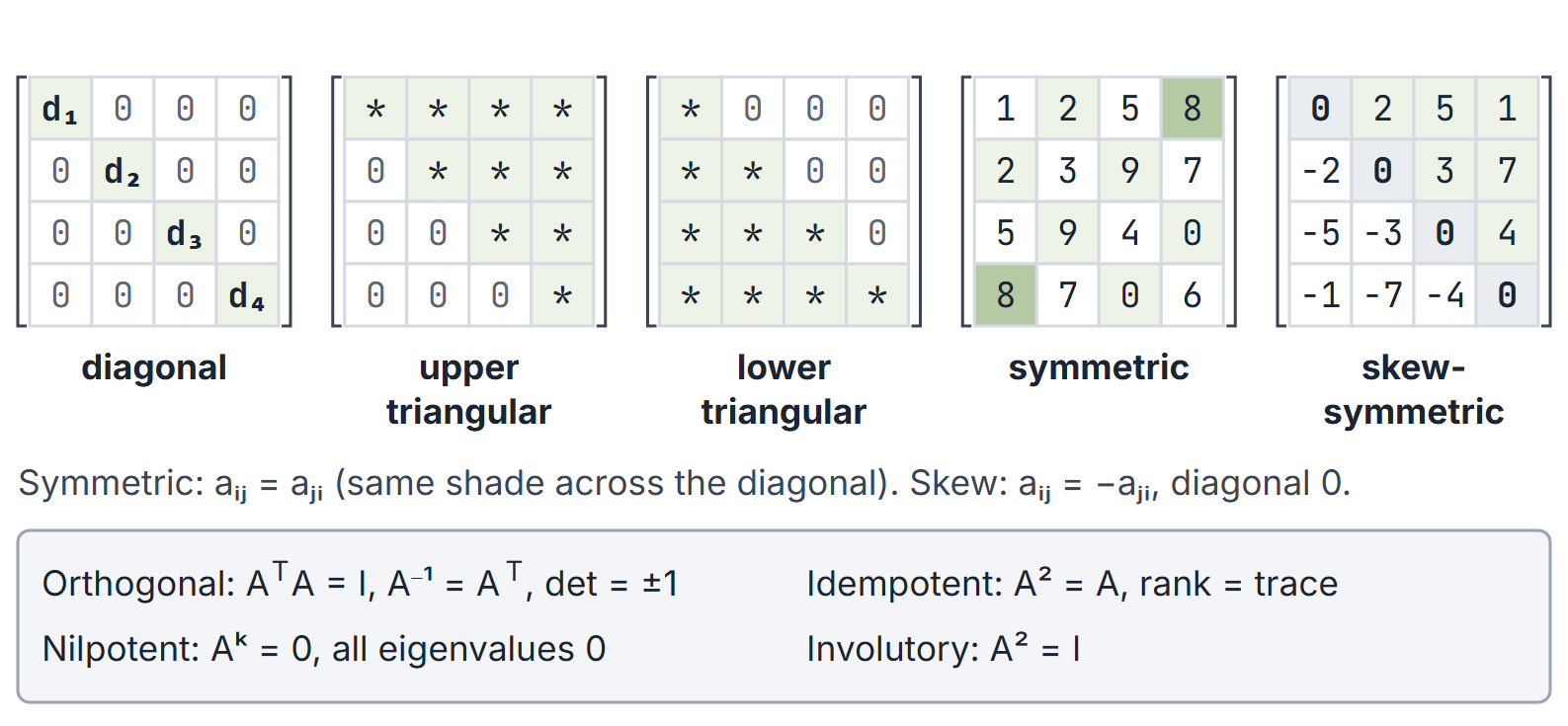
Key facts:

The rank of $A$ is the maximum number of linearly independent rows (equivalently, columns). It is developed with row reduction in Systems of Linear Equations and Rank. Useful facts: $\operatorname{rank}(AB) \le \min(\operatorname{rank} A, \operatorname{rank} B)$ and $\operatorname{rank}(A^T) = \operatorname{rank}(A)$.

More rank facts. For matrices of compatible sizes, $\operatorname{rank}(A + B) \le \operatorname{rank} A + \operatorname{rank} B$; multiplying by invertible matrices does not change rank, $\operatorname{rank}(PAQ) = \operatorname{rank} A$; for real $A$, $\operatorname{rank}(A^TA) = \operatorname{rank}(AA^T) = \operatorname{rank} A$. A non-zero column times a non-zero row, $uv^T$, has rank 1, and every rank-1 matrix has this form.

Trace facts. $\operatorname{tr}(AB) = \operatorname{tr}(BA)$ holds even when $A$ is $m \times n$ and $B$ is $n \times m$, so $AB$ and $BA$ have different sizes. The trace is invariant under cyclic shifts, $\operatorname{tr}(ABC) = \operatorname{tr}(CAB) = \operatorname{tr}(BCA)$, but not under arbitrary reorderings. One consequence: no square matrices satisfy $AB - BA = I$, because the left side has trace 0 and the right side has trace $n$.

$A = \begin{pmatrix} 1 & 2 \\ 3 & 4 \end{pmatrix}$, $B = \begin{pmatrix} 0 & 1 \\ 1 & 0 \end{pmatrix}$. Then $AB = \begin{pmatrix} 2 & 1 \\ 4 & 3 \end{pmatrix}$ (columns swapped) while $BA = \begin{pmatrix} 3 & 4 \\ 1 & 2 \end{pmatrix}$ (rows swapped). Both have trace 5, as $\operatorname{tr}(AB) = \operatorname{tr}(BA)$ predicts.

$A = \begin{pmatrix} 1 & 1 \\ 1 & 1 \end{pmatrix}$, $B = \begin{pmatrix} 1 & -1 \\ -1 & 1 \end{pmatrix}$: $AB = 0$ although neither factor is zero.

$A = \begin{pmatrix} 1 & 4 \\ 2 & 3 \end{pmatrix} = \begin{pmatrix} 1 & 3 \\ 3 & 3 \end{pmatrix} + \begin{pmatrix} 0 & 1 \\ -1 & 0 \end{pmatrix}$.

$\begin{pmatrix} 2 & 1 \\ 5 & 3 \end{pmatrix}$ has determinant $1$, so its inverse is $\begin{pmatrix} 3 & -1 \\ -5 & 2 \end{pmatrix}$. Check by multiplying.

$A = \begin{pmatrix} 1 & 1 \\ 0 & 1 \end{pmatrix}$ gives $A^n = \begin{pmatrix} 1 & n \\ 0 & 1 \end{pmatrix}$ by induction. The idempotent $P = \begin{pmatrix} 1 & 1 \\ 0 & 0 \end{pmatrix}$ satisfies $P^2 = P$, $\operatorname{tr} P = 1 = \operatorname{rank} P$. The rotation $R_\theta = \begin{pmatrix} \cos\theta & -\sin\theta \\ \sin\theta & \cos\theta \end{pmatrix}$ is orthogonal with $R_\theta^{-1} = R_\theta^T = R_{-\theta}$.

$A$ is $10 \times 100$, $B$ is $100 \times 5$, $C$ is $5 \times 50$. $(AB)C$ costs $10 \cdot 100 \cdot 5 + 10 \cdot 5 \cdot 50 = 7500$ multiplications; $A(BC)$ costs $100 \cdot 5 \cdot 50 + 10 \cdot 100 \cdot 50 = 75000$.

An $n \times n$ symmetric matrix is fixed by its entries on and above the diagonal: $n(n + 1)/2$ free entries. With entries from $\{0, 1\}$ there are $2^{n(n+1)/2}$ such matrices (64 for $n = 3$). A skew-symmetric matrix has a zero diagonal and $n(n - 1)/2$ free entries above it; with entries from $\{-1, 0, 1\}$ there are $3^{n(n-1)/2}$ (27 for $n = 3$).

$N = \begin{pmatrix} 0 & 1 & 0 \\ 0 & 0 & 1 \\ 0 & 0 & 0 \end{pmatrix}$ has $N^3 = 0$, so $(I + N)^{-1} = I - N + N^2 = \begin{pmatrix} 1 & -1 & 1 \\ 0 & 1 & -1 \\ 0 & 0 & 1 \end{pmatrix}$.

Let $u = (1, 2, 3)^T$ and $v = (1, 1, 1)^T$, so $A = uv^T$ has rows $(1, 1, 1)$, $(2, 2, 2)$, $(3, 3, 3)$ and rank 1. Since $A^2 = u(v^Tu)v^T = (v^Tu)A$ and $v^Tu = 6 = \operatorname{tr}A$,

so $A^3 = 36A$ and every entry of $A^3$ is 36 times the matching entry of $A$. No matrix multiplication is needed.

$A = \begin{pmatrix} 1 & 2 & 0 \\ 0 & 1 & 3 \end{pmatrix}$ and $B = \begin{pmatrix} 1 & 0 \\ 2 & 1 \\ 0 & 4 \end{pmatrix}$. Then $AB = \begin{pmatrix} 5 & 2 \\ 2 & 13 \end{pmatrix}$ is $2 \times 2$ and $BA = \begin{pmatrix} 1 & 2 & 0 \\ 2 & 5 & 3 \\ 0 & 4 & 12 \end{pmatrix}$ is $3 \times 3$, yet both traces are 18. For a non-cyclic reordering, take the matrix units $E_{12}, E_{21}, E_{11}$ (a single 1 in the named position): $\operatorname{tr}(E_{12}E_{21}E_{11}) = 1$ but $\operatorname{tr}(E_{12}E_{11}E_{21}) = 0$.