LU Decomposition

Gaussian elimination does two jobs at once: it transforms the matrix and it transforms the right-hand side. LU decomposition separates them. It records elimination once as $A = LU$, a lower triangular matrix times an upper triangular one, and then solves $Ax = b$ for any number of right-hand sides with two cheap triangular solves. The tasks are to find the factors of a small matrix, a particular entry of $L$ or $U$, the conditions under which the factorisation exists, or the cost of solving.

For a square matrix $A$, an LU decomposition is $A = LU$ with $L$ lower triangular and $U$ upper triangular. Since $n^2$ entries of $A$ cannot fix the $n^2 + n$ entries of $L$ and $U$, a normalisation is chosen:

Factorisation convention. "LU" means Doolittle unless a question says otherwise.

Run elimination without row swaps. To clear entry $(i, j)$ below the pivot $u_{jj}$, subtract $\ell_{ij} = a^{(j)}_{ij}/u_{jj}$ times row $j$ from row $i$ (with $a^{(j)}$ the current entries). Then

The multipliers go into $L$ with the same sign as they were used for subtraction. Equivalently, the Doolittle formulas compute row $k$ of $U$ and column $k$ of $L$ in turn:

With $A = LU$, write $Ux = y$. Then:

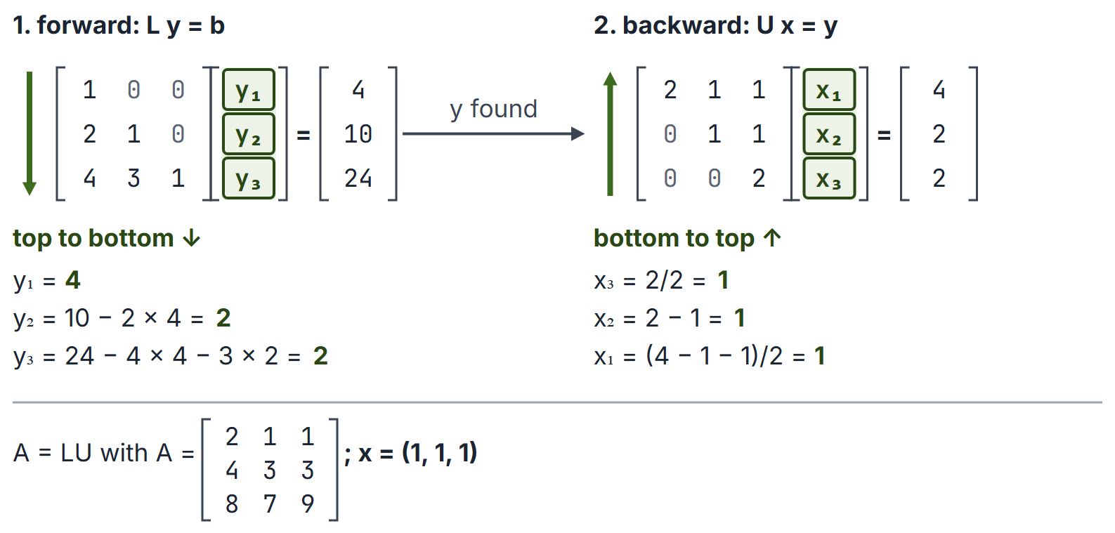
Cost. Factorising an $n \times n$ matrix takes about $n^3/3$ multiplications (and as many additions), that is $O(n^3)$. Each triangular solve takes about $n^2/2$ multiplications, so each additional right-hand side costs only $O(n^2)$. This is why LU is preferred over computing $A^{-1}$ when the same $A$ appears with many $b$.

Determinant for free. $\det A = \det L \cdot \det U = \prod_i u_{ii}$ for Doolittle (and with row swaps, multiply by $(-1)^{\text{number of swaps}}$).

If $A$ is symmetric positive definite ($x^TAx > 0$ for all $x \ne 0$; equivalently all eigenvalues positive; equivalently all leading principal minors positive), then $A = LL^T$ with a unique lower triangular $L$ having positive diagonal. It needs about half the work of LU.

$A = \begin{pmatrix} 2 & 1 & 1 \\ 4 & 3 & 3 \\ 8 & 7 & 9 \end{pmatrix}$, $b = (4, 10, 24)^T$.

Column 1: multipliers $\ell_{21} = 4/2 = 2$, $\ell_{31} = 8/2 = 4$; rows become $(0, 1, 1)$ and $(0, 3, 5)$. Column 2: $\ell_{32} = 3/1 = 3$; row 3 becomes $(0, 0, 2)$. So

Forward: $y_1 = 4$, $y_2 = 10 - 2 \cdot 4 = 2$, $y_3 = 24 - 4 \cdot 4 - 3 \cdot 2 = 2$. Back: $x_3 = 2/2 = 1$, $x_2 = 2 - 1 = 1$, $x_1 = (4 - 1 - 1)/2 = 1$. So $x = (1, 1, 1)$.

$A = \begin{pmatrix} 4 & 3 \\ 6 & 3 \end{pmatrix}$. Doolittle: $L = \begin{pmatrix} 1 & 0 \\ 1.5 & 1 \end{pmatrix}$, $U = \begin{pmatrix} 4 & 3 \\ 0 & -1.5 \end{pmatrix}$. Crout: $L = \begin{pmatrix} 4 & 0 \\ 6 & -1.5 \end{pmatrix}$, $U = \begin{pmatrix} 1 & 0.75 \\ 0 & 1 \end{pmatrix}$. Both multiply back to $A$; both give $\det A = -6$.

$A = \begin{pmatrix} 0 & 1 \\ 1 & 1 \end{pmatrix}$ is invertible, but its first leading minor is 0, so it has no LU decomposition: $\ell_{11}u_{11} = 0$ would force $L$ or $U$ to be singular. Swapping the rows gives $PA = \begin{pmatrix} 1 & 1 \\ 0 & 1 \end{pmatrix} = I \cdot PA$, already upper triangular.

$A = \begin{pmatrix} 2 & 4 \\ 6 & k \end{pmatrix}$: $\ell_{21} = 3$, $u_{22} = k - 12$. The factorisation exists for every $k$ (the first pivot is 2); $A$ is singular exactly when $k = 12$.

$A = \begin{pmatrix} 4 & 2 \\ 2 & 5 \end{pmatrix}$ (leading minors 4 and 16, positive). $\ell_{11} = 2$, $\ell_{21} = 2/2 = 1$, $\ell_{22} = \sqrt{5 - 1} = 2$: $L = \begin{pmatrix} 2 & 0 \\ 1 & 2 \end{pmatrix}$ and $LL^T = A$.

For the matrix of Example 1, the leading principal minors are $\det A_1 = 2$, $\det A_2 = 2 \cdot 3 - 1 \cdot 4 = 2$ and $\det A_3 = 4$. The pivots are therefore $2/1 = 2$, $2/2 = 1$ and $4/2 = 2$, matching the diagonal of $U$ without doing any elimination.

For $n = 1000$ and 100 right-hand sides, repeating elimination costs about $100 \times n^3/3 \approx 3.3 \times 10^{10}$ multiplications. Factoring once and doing two triangular solves per right-hand side costs about $n^3/3 + 100 \times n^2 \approx 3.3 \times 10^8 + 10^8 \approx 4.3 \times 10^8$, roughly 77 times fewer multiplications.

$T = \begin{pmatrix} 2 & -1 & 0 \\ -1 & 2 & -1 \\ 0 & -1 & 2 \end{pmatrix}$. Elimination gives $\ell_{21} = -1/2$, $u_{22} = 3/2$, $\ell_{32} = -2/3$, $u_{33} = 4/3$:

The pivots $2, 3/2, 4/3$ are the ratios $2/1, 3/2, 4/3$ of consecutive leading minors, and $\det T = 2 \cdot \frac32 \cdot \frac43 = 4$. Here all required pivots are nonzero. Under that condition both factors are bidiagonal, so for an $n \times n$ tridiagonal matrix factorisation and each solve take $O(n)$ operations instead of $O(n^3)$ and $O(n^2)$ (the Thomas algorithm). If a required pivot vanishes, use an appropriate pivoted banded solver rather than dividing by zero.

$A = \begin{pmatrix} 0 & 0 \\ 0 & 1 \end{pmatrix}$ has a zero first leading minor, yet for every number $\ell$, $L = \begin{pmatrix} 1 & 0 \\ \ell & 1 \end{pmatrix}$ and $U = \begin{pmatrix} 0 & 0 \\ 0 & 1 \end{pmatrix}$ give $LU = A$. So for singular matrices a zero leading minor does not rule out an LU factorisation, and the factorisation need not be unique; the clean "exists uniquely if and only if the leading minors are non-zero" statement is for invertible matrices.