Systems of Linear Equations and Rank

A system of $m$ linear equations in $n$ unknowns can have exactly one solution, infinitely many, or none. Rank decides which, and Gaussian elimination computes both the rank and the solutions. The rank-nullity theorem then counts how many free parameters a solution set has. These ideas are the core of linear algebra questions: decide for which parameter values a system is consistent, find the rank of a matrix, or count the dimension of a solution space.

The system $a_{i1}x_1 + \cdots + a_{in}x_n = b_i$ ($i = 1, \ldots, m$) is $Ax = b$ with coefficient matrix $A$ ($m \times n$) and augmented matrix $[A \mid b]$ ($m \times (n + 1)$). It is homogeneous if $b = 0$. It is consistent if it has at least one solution.

Vectors $v_1, \ldots, v_k$ are linearly independent if $c_1v_1 + \cdots + c_kv_k = 0$ forces all $c_i = 0$; otherwise dependent. Their span is the set of all linear combinations. A basis of a subspace is an independent spanning set; all bases have the same size, the dimension. In $\mathbb{R}^n$, more than $n$ vectors are always dependent.

For an $m \times n$ matrix $A$:

Three operations do not change the solution set: swap two rows, multiply a row by a non-zero scalar, add a multiple of one row to another. They also preserve the row space and the rank.

A matrix is in row echelon form (REF) if zero rows are at the bottom and the first non-zero entry (pivot) of each row lies strictly to the right of the pivot above it. It is in reduced row echelon form (RREF) if additionally each pivot is 1 and is the only non-zero entry in its column. The RREF of a matrix is unique; REF is not. Gaussian elimination reaches REF and then solves by back substitution; Gauss-Jordan elimination continues to RREF. Both take $O(n^3)$ arithmetic operations for an $n \times n$ system.

The rank of $A$ is any of these equal numbers:

Facts: $\operatorname{rank} A \le \min(m, n)$; $\operatorname{rank} A^T = \operatorname{rank} A$; $\operatorname{rank}(AB) \le \min(\operatorname{rank} A, \operatorname{rank} B)$; multiplying by an invertible matrix does not change rank; $\operatorname{rank}(A^TA) = \operatorname{rank} A$ for real $A$; $\operatorname{rank}(A + B) \le \operatorname{rank} A + \operatorname{rank} B$. A non-zero matrix has rank 1 if and only if it is an outer product $uv^T$ of non-zero vectors.

For an $m \times n$ matrix $A$ (note: $n$ = number of columns = number of unknowns),

Each non-pivot column corresponds to a free variable, and the null space has a basis with one vector per free variable.

Let $r = \operatorname{rank} A$ and $r' = \operatorname{rank}[A \mid b]$. Always $r \le r' \le r + 1$.

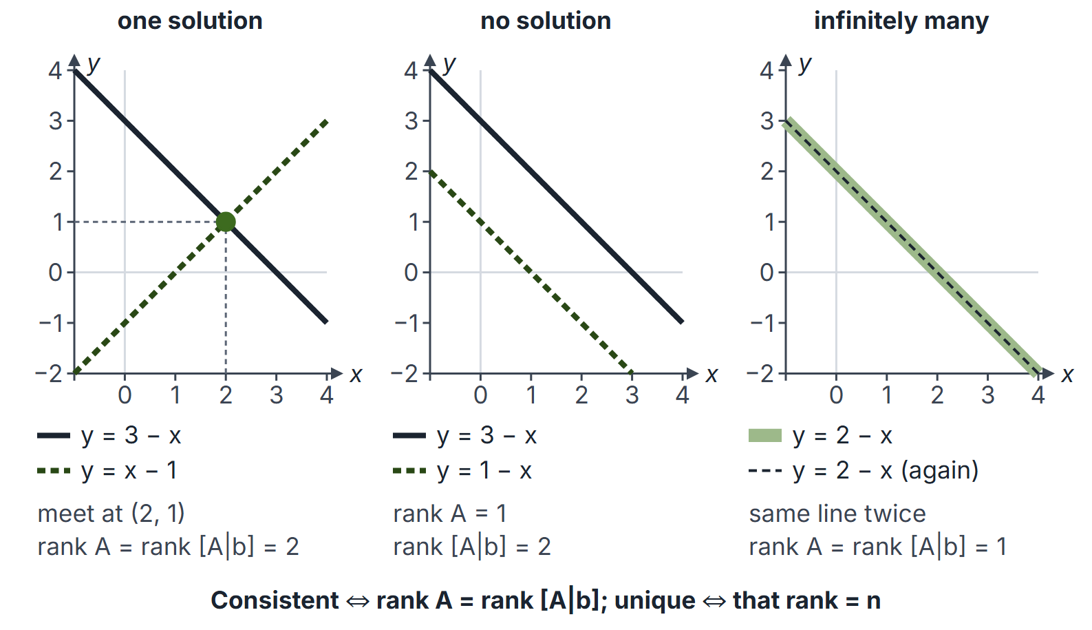
Structure of solutions. If $x_p$ is any one solution of $Ax = b$, then every solution is $x_p + x_h$ with $x_h \in N(A)$. So the solution set, when non-empty, has the same "size" as the null space.

Homogeneous systems $Ax = 0$ are always consistent ($x = 0$). They have a non-trivial solution if and only if $\operatorname{rank} A < n$. In particular:

Square systems. For $n \times n$ $A$, these are equivalent: $\det A \ne 0$; $A$ invertible; $\operatorname{rank} A = n$; $Ax = 0$ has only the trivial solution; $Ax = b$ has a unique solution for every $b$. If $\det A = 0$, then $Ax = b$ has either no solution or infinitely many, depending on $b$; the determinant alone cannot tell which.

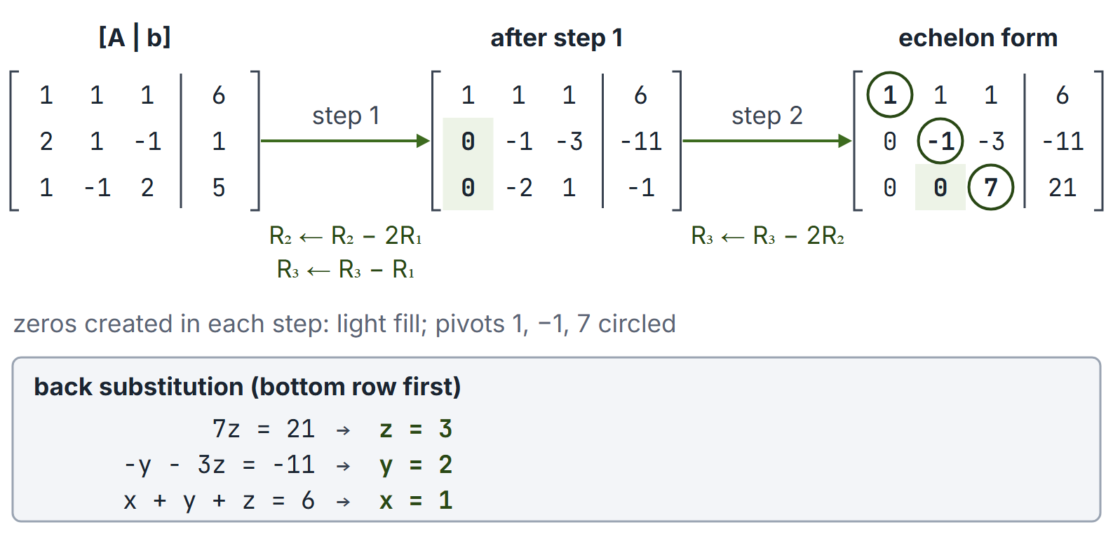
$x + y + z = 6$, $2x + y - z = 1$, $x - y + 2z = 5$. Augmented matrix and operations:

Back substitution: $z = 3$; $-y - 9 = -11$ so $y = 2$; $x = 6 - 2 - 3 = 1$. Rank 3 = $n$: unique.

$x + y + z = 6$, $x + 2y + 3z = 10$, $x + 2y + \lambda z = \mu$. Subtracting gives rows $(0, 1, 2 \mid 4)$ and $(0, 0, \lambda - 3 \mid \mu - 10)$. So:

$x + y + z = 6$, $x + 2y + 3z = 14$, $2x + 3y + 4z = 20$. Row 3 = row 1 + row 2, so $r = r' = 2 < 3$. With $z = t$: $y = 8 - 2t$, $x = -2 + t$. The solution set is the line $(-2, 8, 0) + t(1, -2, 1)$.

$A = \begin{pmatrix} 1 & 2 & 3 & 4 \\ 2 & 4 & 6 & 8 \\ 1 & 0 & 1 & 0 \end{pmatrix}$. Row 2 is twice row 1, and rows 1 and 3 are independent: rank 2. Nullity $= 4 - 2 = 2$, so $Ax = 0$ has a two-parameter family of solutions.

$x + ky = 0$, $kx + y = 0$ has a non-trivial solution if and only if $\det = 1 - k^2 = 0$, that is $k = \pm 1$.

For $n \ge 2$, the $n \times n$ matrices with entries $a_{ij} = i + j$ and with entries $1, 2, \ldots, n^2$ filled row by row both have rank 2: every row is a combination of $(1, 1, \ldots, 1)$ and $(1, 2, \ldots, n)$. The matrix with $a_{ij} = ij$ has rank 1, because row $i$ is $i$ times row 1. Rank-nullity then gives null spaces of dimension $n - 2$ and $n - 1$.

Over GF(2) (arithmetic modulo 2), solve $x_1 + x_2 + x_3 = 1$, $x_2 + x_3 = 0$. The coefficient matrix has rank 2 and so does the augmented matrix, with $n = 3$ unknowns, so there are $2^{3 - 2} = 2$ solutions: $x_3$ is free, $x_2 = x_3$, $x_1 = 1$, giving $(1, 0, 0)$ and $(1, 1, 1)$.