
Introduction
Most vectors change direction when a matrix acts on them. Eigenvectors are the special non-zero vectors whose direction is preserved (or exactly reversed) for a nonzero real eigenvalue, or which are collapsed to zero for eigenvalue 0; complex eigenvectors are understood through the algebraic equation below. The matrix scales an eigenvector, by a factor called the eigenvalue. Eigenvalues summarise a matrix compactly: their sum is the trace, their product is the determinant, and they decide invertibility, powers, stability and diagonalisability. Many eigenvalue facts follow from properties alone, without solving a cubic.
Prerequisites
- Determinants: , triangular determinants, .
- Systems of Linear Equations and Rank: null space, rank-nullity, homogeneous systems.
Core concepts
Definition
Let be . A scalar is an eigenvalue of if there is a non-zero vector with
Such is an eigenvector for . The zero vector is never an eigenvector, but can be an eigenvalue. Rewriting as , a non-zero solution exists if and only if is singular:
is a polynomial of degree (some books use , which differs by the factor and has the same roots). Over it has exactly roots counted with multiplicity; a real matrix can have complex eigenvalues, which come in conjugate pairs. The eigenspace of is : all eigenvectors for together with .
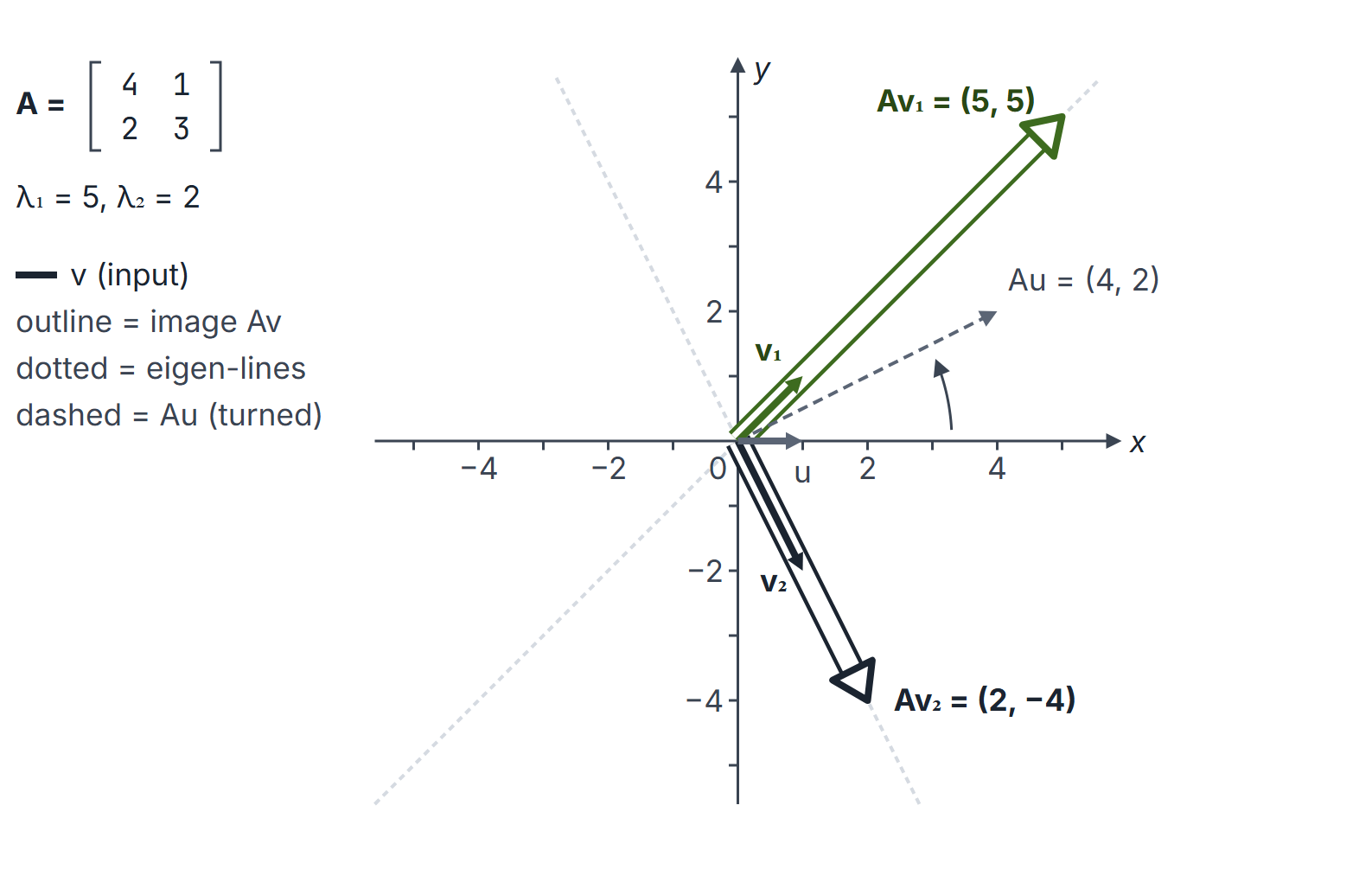
Trace, determinant and the shortcut
If the eigenvalues (with algebraic multiplicity) are , then
For : . Consequently, is singular if and only if 0 is an eigenvalue.
Multiplicities
- Algebraic multiplicity (AM) of : its multiplicity as a root of .
- Geometric multiplicity (GM) of : .
Always .
Eigenvalues of related matrices
If , then with the same eigenvector :
| Matrix | Eigenvalue |
|---|---|
| () | |
| (if invertible) | |
| polynomial | |
| (if invertible) |
Also: has the same eigenvalues as (same characteristic polynomial) but generally different eigenvectors; and have the same eigenvalues for square ; similar matrices share the characteristic polynomial, hence eigenvalues, trace, determinant and rank. Eigenvalues of are not sums of eigenvalues of and in general.
Triangular and diagonal matrices: the eigenvalues are the diagonal entries.
Eigenvalues of special matrices
| Matrix (real) | Eigenvalues |
|---|---|
| Symmetric | all real; eigenvectors of distinct eigenvalues are orthogonal |
| Skew-symmetric | zero or purely imaginary |
| Orthogonal | modulus 1 (real ones are ) |
| Idempotent | 0 or 1 |
| Nilpotent | all 0 |
| Involutory | |
| Stochastic (non-negative, rows sum to 1) | 1 is an eigenvalue (eigenvector all-ones); all have modulus at most 1 |
Diagonalisation
is diagonalisable if with diagonal; the columns of are eigenvectors and the diagonal of holds the matching eigenvalues.
- Necessary and sufficient: has linearly independent eigenvectors; equivalently, GM = AM for every eigenvalue.
- Sufficient, not necessary: distinct eigenvalues (eigenvectors of distinct eigenvalues are independent). The identity has one repeated eigenvalue yet is diagonal.
- Sufficient: real symmetric. Then with orthogonal (spectral theorem).
- Not diagonalisable: any eigenvalue with GM AM, for example .
Diagonalisation makes powers easy: .
Cayley-Hamilton theorem
Every square matrix satisfies its own characteristic equation: if , then . For : . Uses: express or high powers of as a polynomial of degree less than in .
Rank and eigenvalues
The geometric multiplicity of the eigenvalue 0 is . Since GM AM, the number of non-zero eigenvalues counted with algebraic multiplicity, with equality when is diagonalisable. Equality can fail otherwise: The nilpotent has rank 1 but no non-zero eigenvalue.
Quadratic forms and positive definiteness
A real symmetric is positive definite if for every . The following are equivalent: is positive definite; all eigenvalues of are positive; all leading principal minors of are positive (Sylvester's criterion); with lower triangular with positive diagonal (Cholesky, see LU Decomposition). Positive semidefinite means , equivalently all eigenvalues ; for this weaker property the leading minors are not enough: has leading minors 0 and 0 but eigenvalue .
Worked examples
Example 1: a matrix
: trace 7, determinant 10, so , . For : , eigenvector . For : , eigenvector . With , ; for instance, the entry of is .
Example 2: defective matrix
. Eigenvalues . has rank 2, so GM(2) = 1 AM(2) = 2: not diagonalisable.
Example 3: properties only
A matrix has eigenvalues . Then , ; has ; has and is singular; has and determinant . is diagonalisable (distinct eigenvalues).
Example 4: Cayley-Hamilton
: . Multiply by : .
Example 5: symmetric and rotation matrices
has eigenvalues 3 and 1 with orthogonal eigenvectors and . The rotation by , , has , so : no real eigenvector, as expected since every direction turns.
Example 6: the all-ones matrix
(every entry 1) has rank 1, so 0 has GM ; the trace must be the remaining eigenvalue, with eigenvector . Eigenvalues: once, with multiplicity . Hence has eigenvalues and ( times), and .
Example 7: powers by diagonalisation
: trace 7, determinant 10, so , with eigenvectors and . With and ,
For this returns ; for it gives . For large , : the largest eigenvalue dominates.
Example 8: a positive definite tridiagonal matrix
has leading principal minors , all positive, so is positive definite. Its eigenvalues are , , , all positive; their sum is and their product is . The sum of their squares is , not .
Important properties and observations
- Row operations change eigenvalues; never row-reduce before finding its eigenvalues.
- Eigenvectors are determined only up to non-zero scalar multiples; any multiple is an equally valid answer.
- If every row of sums to , then is an eigenvalue with eigenvector .
- A real matrix with odd has at least one real eigenvalue.
GATE examination perspective
- Trace and determinant to find a missing eigenvalue, or the eigenvalues of a matrix.
- Eigenvalues of , , , polynomials in , adjugates.
- Diagonalisability via GM versus AM; counting independent eigenvectors.
- Special matrices: triangular, symmetric, idempotent, rank-one, all-ones.
- Cayley-Hamilton for inverses and powers.
- Trap: taking " distinct eigenvalues" as necessary for diagonalisability.
- Trap: adding eigenvalues of and to get those of .
- Definiteness. Symmetric is positive definite iff all leading principal minors are positive, iff all eigenvalues are positive.
- Trap: , which is not .
Summary
Sources
- G. Strang, Introduction to Linear Algebra, 5th ed., Wellesley-Cambridge Press, 2016: Chapter 6 (Eigenvalues and Eigenvectors), Sections 6.1 (Introduction to Eigenvalues), 6.2 (Diagonalizing a Matrix) and 6.4 (Symmetric Matrices).
- E. Kreyszig, Advanced Engineering Mathematics, 10th ed., Wiley, 2011: Chapter 8 (Linear Algebra: Matrix Eigenvalue Problems).