
Introduction
A graph is a set of vertices and a set of edges , each edge joining two vertices. Graphs model road networks, links between web pages, dependencies between tasks and much more. Before any graph algorithm can run, the graph must be stored, and the choice of representation fixes the cost of the basic questions: "is there an edge from to ?" and "what are the neighbours of ?".
This note covers the adjacency matrix, the adjacency list, and the edge list and incidence matrix, with their space and time costs and the facts that follow from them. The graph theory itself (paths, connectivity, special graphs) is in Graph Theory Fundamentals; traversals are in Breadth-First Search and Depth-First Search.
Conventions: , ; vertices are numbered ; graphs are simple (no self-loops, no parallel edges) unless stated. An adjacency matrix or array of lists is 0-based unless a question states 1-based numbering. Linked adjacency lists use pointers, not array indices.
Prerequisites
- Graph Theory Fundamentals: vertices, edges, degree, directed and undirected graphs.
- Linked Lists: adjacency lists are linked lists.
- Arrays: Address Calculation and Special Matrices: two-dimensional arrays.
Core concepts
Terminology needed here
- In an undirected graph, edge makes and adjacent; the degree is the number of incident edges.
- In a directed graph, edge goes from to ; has out-degree and in-degree.
- Handshake lemma: (undirected); (directed).
- A simple undirected graph has at most edges; a simple directed graph at most .
- Dense: close to . Sparse: much smaller than , for example .
Running example
Undirected graph with and the edges . Degrees: 2, 3, 2, 2, 1, summing to .
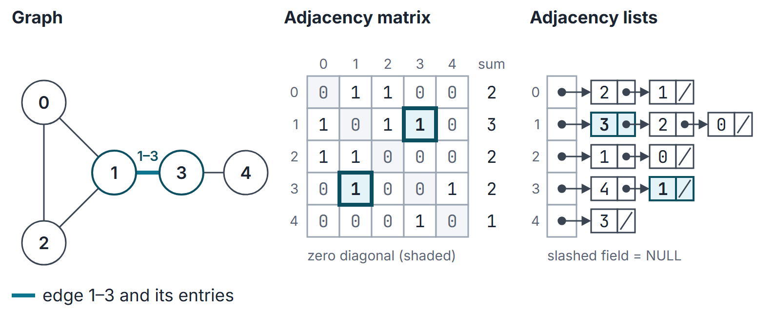
Adjacency matrix
An adjacency matrix stores 1 for an unweighted edge and 0 otherwise. For a weighted graph, store the edge weight and a distinct “no edge” sentinel outside the permitted weight domain, or track presence separately. Zero is a valid sentinel only if every edge weight is nonzero; works only when it is excluded as a genuine edge weight.
For the running example:
- Undirected graph: is symmetric; only the upper triangle needs storing ( entries without the diagonal; see triangular storage).
- Simple graph: zero diagonal.
- Row sum of row = degree (undirected) or out-degree (directed); column sum = in-degree.
- The transpose represents the graph with every edge reversed.
- Powers: the entry is the number of walks of length exactly from to . In the example (the walk 0, 1, 3), and the diagonal of is the degree sequence. The number of triangles in a simple undirected graph is ; here it is 1 (vertices 0, 1, 2).
Adjacency list
An array of lists; the list for holds every adjacent to (for a directed graph, every with an edge ).
struct edge { int to; struct edge *next; };        /* add an int weight field if weighted */
struct edge *adj[V];                                /* adj[u]: head of u's list */

void add(int u, int v) {                            /* insert at head: O(1) */
    struct edge *e = malloc(sizeof *e);             /* allocation check omitted for brevity */
    e->to = v; e->next = adj[u]; adj[u] = e;
}
/* undirected edge {u, v}: add(u, v); add(v, u); */
Inserting at the head, edges added in the order given produce these lists for the running example:
0: 2 1
1: 3 2 0
2: 1 0
3: 4 1
4: 3
The order of vertices inside a list depends on insertion order, and traversal algorithms visit neighbours in list order. A question that asks for a BFS or DFS order "using adjacency lists" therefore depends on how the lists were built; read the stated order.
- Total list entries: for undirected graphs, for directed graphs.
- Length of the list of = degree (out-degree for directed).
- Finding the in-degree of in a directed graph needs a scan of all lists: .
- The reversed graph is built from the lists in .
Edge list and incidence matrix
- Edge list: an array of the pairs (with weights). Space . Natural for Kruskal's algorithm, which sorts edges by weight (Minimum Spanning Trees).
- Incidence matrix: , entry 1 if the vertex is an endpoint of the edge. Each column of an undirected incidence matrix has exactly two 1s; row sums are the degrees. With the incidence matrix, , where is the diagonal matrix of degrees. Rarely used for algorithms because it costs space.
How it works: choosing a representation
| Question or cost | Adjacency matrix | Adjacency list |
|---|---|---|
| Space | ||
| Is an edge? | ||
| List the neighbours of | ||
| Visit every edge (BFS, DFS) | ||
| Add an edge | at the head | |
| Delete directed edge | , searching the outgoing list | |
| Delete undirected edge | without cross pointers: remove both list records | |
| Add a vertex | to rebuild | amortised |
- Sparse graphs (most real graphs, trees, planar graphs) favour lists: space and traversal.
- Dense graphs, or algorithms that need many edge tests (for example Floyd-Warshall all-pairs shortest paths), favour the matrix.
- BFS and DFS cost with lists and with a matrix, because scanning a matrix row costs no matter how few neighbours there are.
For a tree with vertices () the matrix stores entries of which only are 1; the lists store entries.
Worked examples
The adjacency lists used below are the ones built by the add function above (head insertion, edges in the order given).
Example 1. Running example: row sums of are 2, 3, 2, 2, 1; total ; the lists contain entries; the matrix has cells.
Example 2 (directed graph). , edges . Out-degrees 2, 1, 2, 0; in-degrees 1, 1, 2, 1; both sum to . In the transpose, row 2 has 1s in columns 0 and 1 (the edges into vertex 2 were from 0 and 1).
Example 3 (walks). In the running example, (walk 0, 2, 1) and (walk 2, 1, 3); , giving one triangle.
Example 4 (incidence). The 5 by 5 incidence matrix of the running example has two 1s in every column and row sums 2, 3, 2, 2, 1.
Important properties and observations
- Matrix: space regardless of ; edge test.
- Lists: space; neighbour iteration proportional to degree.
- An undirected graph's matrix is symmetric; each undirected edge appears twice in the lists.
- The order of entries in each adjacency list decides tie-breaking in BFS and DFS.
- counts walks of length ; counts triangles in a simple undirected graph.
GATE examination perspective
- Space or time with a given representation: BFS or DFS is with lists, with a matrix.
- Degrees and edge counts from a matrix or from lists, using the handshake lemma.
- Traversal orders that depend on adjacency list order.
- Matrix facts: symmetry, row and column sums, transpose, powers counting walks.
- Dense versus sparse choice for a stated algorithm.
Summary
Sources
- T. H. Cormen, C. E. Leiserson, R. L. Rivest, C. Stein, Introduction to Algorithms, 3rd ed., MIT Press, 2009: Section 22.1 (representations of graphs: adjacency lists and adjacency matrix, transpose, incidence matrix in the exercises).
- K. H. Rosen, Discrete Mathematics and Its Applications, 7th ed., McGraw-Hill, 2012: Section 10.3 (representing graphs, adjacency and incidence matrices) and Section 10.4 (counting paths with powers of the adjacency matrix).