
Introduction
An array stores elements of one type in consecutive memory locations, so the address of any element can be computed from its indices with a little arithmetic. That computation gives access by index, the property that makes arrays the foundation of heaps, hash tables, matrices and dynamic programming tables.
This note centres on address calculations: given the base address, element size, index bounds and storage order, find the address of an element. A second topic is how to store special matrices (triangular, symmetric, tridiagonal, sparse) compactly and where a given element lands. This note derives the general formulas and checks each one by enumeration. How C arrays relate to pointers is in Arrays and Their Relation to Pointers.
Conventions: is the base address (address of the first element), the size of one element in bytes (addressing is by bytes unless addresses are counted in words). Index ranges are written , so a dimension has elements. C arrays always start at index 0; other lower bounds come from languages such as Pascal and Fortran, and from 1-based presentations.
Prerequisites
- Arrays and Their Relation to Pointers: row-major layout of C arrays,
sizeof.
Core concepts
One-dimensional arrays
For A[l..u]:
In C () this is B + i * sizeof A[0], exactly what &A[i] computes.
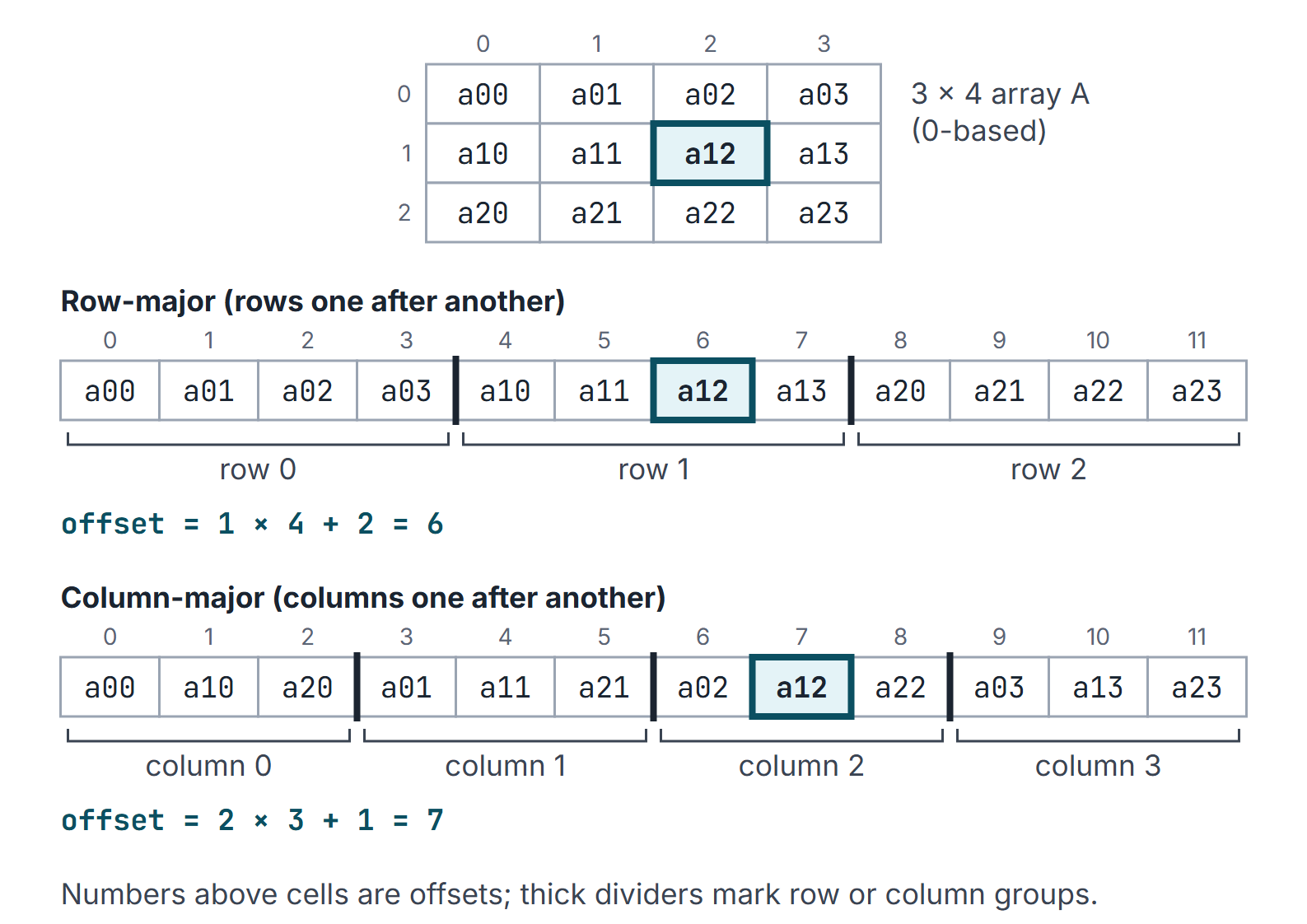
Two-dimensional arrays: row-major and column-major
For A[l1..u1][l2..u2] with rows and columns:
- Row-major (C, C++, Pascal): all of row , then row , and so on.
- Column-major (Fortran, MATLAB): all of column , then the next column, and so on.
In words: count how many complete rows (or columns) come before the element, multiply by the row (or column) length, and add the position inside the current row (or column).
Three or more dimensions
For A[l1..u1][l2..u2][l3..u3] in row-major order, with :
The pattern generalises: in row-major order the last index varies fastest; in column-major order the first index varies fastest. The first dimension's size never appears in the row-major formula, which is why a C function parameter can omit only the first dimension (int a[][4]).
How it works: special matrices
Square matrices with many guaranteed zeros (or repeated entries) can be stored in a one-dimensional array holding only the significant entries. In this section indices are 1-based, , and the formulas give the 0-based offset into the 1D array; the address is .
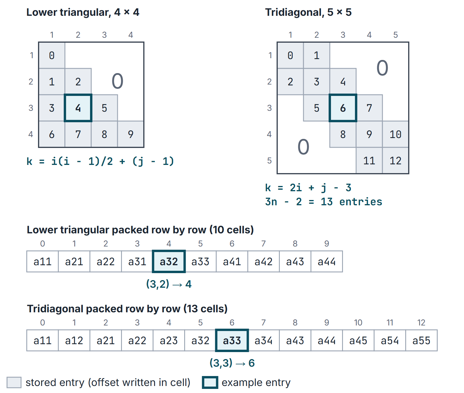
Lower triangular matrix ( for )
Number of stored entries: .
- Row-major: rows contain entries, so
- Column-major: columns contain entries, so
Upper triangular matrix ( for )
- Row-major: , for .
- Column-major: , for .
Note the symmetry: upper triangular column-major has the same shape of formula as lower triangular row-major with and exchanged.
Symmetric matrix ()
Store only the lower triangle ( entries) and access with as .
Tridiagonal and band matrices
A tridiagonal matrix has non-zero entries only where : the main diagonal and the diagonals directly above and below. It has such entries. Stored row by row (row 1 has 2 entries, rows 2 to have 3, row has 2):
A band matrix of positive order and integer half-width , with nonzeros allowed only where , has allowed positions. Tridiagonal is for . If a redundant larger width is supplied, use in the formula.
Sparse matrices
When only a few entries are non-zero but with no fixed pattern, store a list of triplets (row, column, value), usually sorted by row and then column, or use linked lists per row. For non-zero entries the triplet form uses values instead of ; it saves space when (counting each stored value as one unit).
Worked examples
The C row-major offsets below are for C11 with gcc on x86-64 Linux (LP64, 4-byte int).
Example 1 (2D with non-zero lower bounds). A[-3..4][5..10] of 4-byte integers, . Then , .
- Row-major: .
- Column-major: .
The C check models the array as int M[8][6] with A[i][j] at M[i+3][j-5]; the byte offset of M[4][2] is 104, and sizeof M is 192.
Example 2 (3D). A[1..3][1..4][1..5] of 2-byte elements, row-major, : . In C, &T[1][2][3] in int T[3][4][5] is 33 elements from the start.
Example 3 (lower triangular, ). Element : row-major offset ; column-major offset . The packed array has entries; a strictly lower triangular matrix (zero diagonal too) would need .
Example 4 (tridiagonal). For any , is at offset 0, at , and at .
Important properties and observations
- Access by index is because the address is a fixed formula of the indices.
- Insertion or deletion in the middle of an array costs element moves; a linked list avoids the moves but loses indexing.
- Searching an unsorted array is ; a sorted array supports binary search in (Searching).
- Traversing a 2D array in its storage order (row by row for C) touches memory sequentially, which matters for caches (Arrays and Their Relation to Pointers).
- A complete binary tree stored in an array uses index arithmetic in the same spirit: children of index at and in a 1-based heap (Binary Heaps).
- When a question gives addresses in words rather than bytes, take in words.
GATE examination perspective
- Address of an element for given bounds, element size, base and order.
- Reverse problems: given the addresses of two elements, find the base address or a dimension.
- Triangular, symmetric and tridiagonal storage: number of entries, and the offset of a given element in row- or column-major packing.
- Row-major versus column-major in a loop nest: which order of loops accesses memory sequentially.
- Sparse matrices: triplet representation and its space.
Summary
Sources
- D. E. Knuth, The Art of Computer Programming, Vol. 1, 3rd ed., Addison-Wesley, 1997: Section 2.2.6 (arrays and orthogonal lists: sequential allocation of arrays, triangular matrices).
- ISO/IEC 9899:2011 (C11), committee draft N1570, (consulted 2026-11-09): Section 6.5.2.1p3 (multidimensional arrays are stored in row-major order).