Depth-First Search and Edge Classification

Depth-first search (DFS) explores a graph by going as deep as possible along each path before backtracking. It assigns every vertex a discovery time $d[u]$ and a finish time $f[u]$, and it classifies every edge as a tree, back, forward or cross edge. Those timestamps and edge types are the foundation of topological sort and strongly connected components.

Where BFS expands by layers with a queue, DFS expands by a stack (explicit or the call stack). Both run in $\Theta(V+E)$ time on adjacency lists; they answer different questions.

A global clock time starts at 0. When DFS first discovers $u$ it sets $d[u]$ and paints $u$ grey; when it finishes scanning $Adj[u]$ it sets $f[u]$ and paints $u$ black. Every vertex gets a unique pair with $d[u] < f[u]$, and the intervals $[d[u], f[u]]$ nest or are disjoint (parenthesis theorem).

When DFS examines edge $(u,v)$:

The timestamp column (CLRS Exercise 22.3-5) classifies an edge after the search has finished. Tree and forward edges have the same timestamp pattern; they differ only in whether $v$ was discovered through this edge. A cross edge always points to a vertex that was discovered and finished earlier, so it goes "right to left" in a drawing whose trees are ordered by discovery.

In an undirected graph every edge is tree or back (forward and cross do not arise under the standard undirected classification: a non-tree edge always leads to a grey ancestor).

For any two vertices $u,v$, exactly one of the following holds:

Crossing (partly overlapping) intervals such as $d[u] < d[v] < f[u] < f[v]$ never occur.

Subtree size from timestamps. Each vertex receives exactly two timestamps, and all of $u$'s descendants receive theirs between $d[u]$ and $f[u]$. Hence $f[u] - d[u] + 1 = 2 \times$ (number of vertices in $u$'s DFS subtree, $u$ included), whatever the non-tree edges are.

Pseudocode uses adjacency lists, <- for assignment and a global time.

Input. Graph $G=(V,E)$, directed or undirected.

Output. Discovery and finish times, predecessors $\pi$ forming a DFS forest, and (by the colour of the head when an edge is examined) an edge classification.

Time / space. $\Theta(V+E)$ on adjacency lists: each vertex and each edge is processed a constant number of times. Stack depth $O(V)$ in the worst case (a path). Extra space $\Theta(V)$ for colours and timestamps.

Edge cases. Disconnected graphs produce a forest (outer loop starts a new tree at each white vertex). Self-loops in a directed graph are back edges. The forest (and edge types that depend on discovery order) depends on the order of vertices in the outer loop and inside adjacency lists; the parenthesis structure always holds.

At any moment the grey vertices on the call stack form a tree path from the root of the current DFS tree to the vertex now being explored. Discovering a white neighbour extends that path; finishing a vertex pops it. An explicit-stack implementation pushes a frame with the next adjacency-list index and obtains the same forest, which is useful when the language limits recursion depth.

The discovery time of a vertex is the step at which it first becomes grey; the finish time is the step at which it becomes black. Between those two times every descendant is discovered and finished, which is exactly the parenthesis theorem.

Vertex $v$ is a descendant of $u$ in the DFS forest if and only if, at the time $d[u]$, there is a path from $u$ to $v$ consisting entirely of white vertices. This characterises the tree edges DFS will grow.

A path is not enough. A path from $u$ to $v$ together with $d[u] < d[v]$ does not make $v$ a descendant of $u$ (CLRS Exercise 22.3-8). Edges $w \to u$, $u \to w$, $w \to v$, with DFS from $w$ and $Adj[w] = u, v$: DFS discovers $w$ (1), then $u$ (2), sees $u \to w$ as a back edge, finishes $u$ (3), then discovers $v$ (4). The path $u \to w \to v$ exists and $d[u] = 2 < 4 = d[v]$, but $v$ is not a descendant of $u$: when $u$ was discovered, the path went through the grey vertex $w$.

A directed graph has a cycle if and only if DFS finds a back edge. An undirected graph has a cycle if and only if DFS finds a back edge (to a grey ancestor other than the immediate parent, depending on how undirected adjacency is represented).

DFS is not analysed by the master theorem; the $\Theta(V+E)$ bound follows from an aggregate count: the body of DFS-VISIT runs once per vertex, and the adjacency-list scan touches each edge once (twice in undirected representations that store both directions).

Vertices $u,v,w,x$. Edges: $u\to v$, $u\to w$, $v\to w$, $w\to x$, $x\to v$. Outer loop order $u,v,w,x$; adjacency lists in alphabetical order.

DFS starting at $u$:

Timestamps: $d/f = u:1/8,\; v:2/7,\; w:3/6,\; x:4/5$. The edge $x\to v$ is a back edge, so the graph has a cycle $v\to w\to x\to v$.

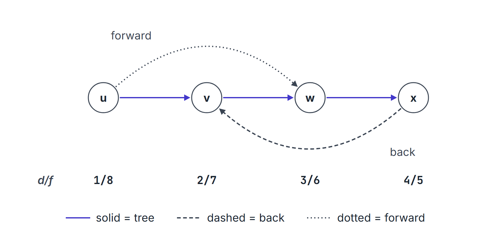
Subtree check: $f[u] - d[u] + 1 = 8 = 2 \times 4$ and $f[w] - d[w] + 1 = 4 = 2 \times 2$ ($w$ and $x$).

Adding a cross edge. Add a fifth vertex $y$ with the single edge $y \to u$, placed last in the outer loop. After $u$'s tree finishes at time 8, the outer loop starts a new tree at $y$: $d[y] = 9$. Edge $y \to u$ finds $u$ black with $d[u] = 1 < 9$, so it is a cross edge, and $f[y] = 10$. If instead $y$ came first in the outer loop, $y \to u$ would be a tree edge and all five vertices would form one tree. Edge types depend on the vertex order.

Use the undirected graph of the BFS note: edges $s{-}a$, $s{-}b$, $a{-}c$, $b{-}c$, $b{-}d$, $c{-}e$, $d{-}e$. Over every ordering of the adjacency lists, DFS from $s$ can discover vertices in exactly five orders: $s,a,c,b,d,e$; $s,a,c,e,d,b$; $s,b,c,a,e,d$; $s,b,c,e,d,a$; $s,b,d,e,c,a$. The order $s,a,c,e,b,d$ is impossible: after $e$ is discovered, $e$ still has the white neighbour $d$, so DFS must go to $d$ before backtracking to $c$. IMPERATIVE RULE. The next discovered vertex must be a white neighbour of the deepest grey vertex that still has a white neighbour.

Triangle $a{-}b{-}c{-}a$. DFS from $a$ with lists $b,c$ for $a$: tree edges $a{-}b$, $b{-}c$; the edge $c{-}a$ is a back edge to the grey ancestor $a$. Finish order $c,b,a$.

Discovery order is a preorder walk of the DFS forest: a vertex is listed before its descendants. Finish order is a postorder walk: a vertex is listed after its descendants. Topological sort of a DAG is exactly the reverse of the finish order, which is why a single DFS suffices when the graph has no back edges.

Common misconceptions.