Breadth-First Search

Breadth-first search (BFS) explores a graph level by level from a source $s$: it visits every vertex at distance $k$ before any vertex at distance $k+1$. The search builds a BFS tree of shortest paths in the unweighted sense (fewest edges) and assigns each reachable vertex a distance $d[v] = \delta(s,v)$.

BFS is the standard first algorithm on unweighted graphs: it needs a queue, runs in $\Theta(V+E)$ time on an adjacency-list representation, and is the template for unweighted shortest paths and for bipartiteness testing. The same layer order underlies several standard applications: testing whether an undirected graph is bipartite, computing the eccentricity of a vertex, and (with two passes) the diameter of a tree. Weighted graphs need different algorithms; BFS is the unweighted base case that those algorithms generalise.

CLRS colours vertices white (undiscovered), grey (discovered but not fully explored) and black (fully explored). A single bit (discovered or not) suffices for correctness of distances; grey versus black is pedagogical.

On termination, for every vertex $v$ reachable from $s$:

the fewest edges on any $s$--$v$ path, and the predecessor $\pi[v]$ yields a shortest path by walking $\pi$ to $s$. Unreachable vertices keep $d[v] = \infty$ and $\pi[v] = \mathrm{NIL}$.

The vertices with $d[v] = k$ form layer $k$. Every edge of the BFS tree joins consecutive layers.

Edge rule. For every edge $(u,v)$ of a graph explored from $s$, with $u$ reachable, $d[v] \le d[u] + 1$: when $u$ is dequeued, $v$ is either discovered then at distance $d[u]+1$ or was already discovered at a smaller or equal distance.

Pseudocode uses adjacency lists Adj[u], <- for assignment and a FIFO queue Q.

Input. Graph $G=(V,E)$ (directed or undirected) and source $s \in V$.

Output. Attributes $d$ and $\pi$ on $V$; the BFS tree edges are $\{( \pi[v], v) : \pi[v] \ne \mathrm{NIL}\}$.

Time / space. Each vertex is enqueued at most once and each adjacency list is scanned once: $\Theta(V+E)$ on adjacency lists. On an adjacency matrix the neighbour scan costs $\Theta(V^2)$. Extra space $\Theta(V)$ for colours, distances, predecessors and the queue.

Edge cases. Isolated source: $d[s]=0$, all others $\infty$. Self-loops and parallel edges do not change distances. In a disconnected undirected graph, BFS from $s$ reaches only $s$'s component; a full covering needs a loop over unused sources (as in DFS).

Queued grey vertices await processing; the currently scanned grey vertex has already left the queue and becomes black only after its adjacency scan finishes. Newly discovered neighbours are enqueued at the back; the next vertex to explore is taken from the front. That FIFO discipline is exactly what forces layer $k$ to finish before layer $k+1$ begins. Replacing the queue by a stack yields a form of DFS and destroys the distance guarantee.

Space for the queue is $O(V)$ in the worst case (for example a star: the centre discovers all leaves before any leaf is dequeued). The queue contains vertices from at most two consecutive distance layers. If the maximum reachable layer width is $W$, its peak size is at least $W$ and at most $2W$, hence $O(V)$, not necessarily exactly $W$. For example, let the source discover $a,b,c$, and let $a$ discover $d,e,f$. Both nontrivial layers have width 3, but after exploring $a$ the queue is $b,c,d,e,f$, of size 5.

A standard inductive argument (CLRS 3e, Section 22.2) shows that when a vertex $v$ is first discovered from $u$, one has $d[v] = d[u]+1 = \delta(s,v)$. The queue always holds vertices of at most two consecutive distances, so layers are processed in order.

An undirected graph is bipartite if and only if it has no odd cycle. Run BFS from each undiscovered source and try to 2-colour by layer parity ($d[v] \bmod 2$). Because every edge joins equal or adjacent layers, the colouring fails exactly when some edge joins two vertices of the same layer. Such an edge $(u,v)$ closes an odd cycle: the tree paths from $u$ and from $v$ up to their lowest common ancestor have equal length, so together with the edge they form a cycle of odd length. Time still $\Theta(V+E)$.

BFS also counts fewest-edge paths. Before BFS, initialize $cnt[v]=0$ for every vertex, then set $cnt[s]=1$. When $u$ is dequeued, for each neighbour $v$ with $d[v] = d[u] + 1$ (just discovered or discovered earlier in this layer), add $cnt[u]$ to $cnt[v]$. Because a whole layer is dequeued before the next, $cnt[u]$ is final when it is used.

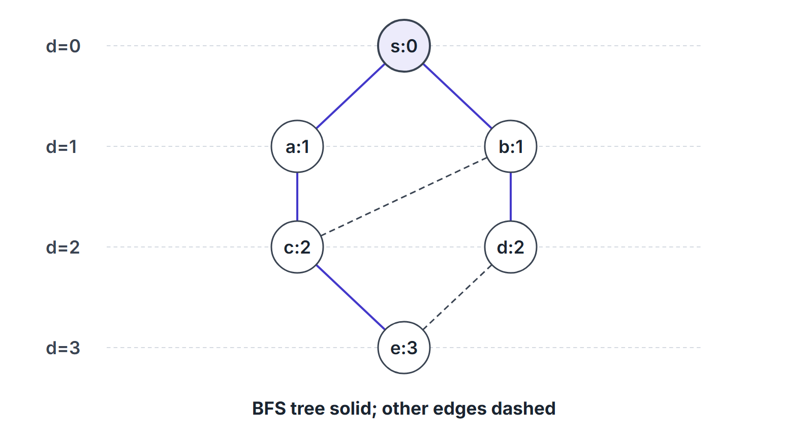
Vertices $\{s,a,b,c,d,e\}$. Edges: $s{-}a$, $s{-}b$, $a{-}c$, $b{-}c$, $b{-}d$, $c{-}e$, $d{-}e$. Adjacency lists in alphabetical order within each list, with $s$ first in its own list written as $a,b$.

BFS from $s$:

Distances: $s:0$, $a:1$, $b:1$, $c:2$, $d:2$, $e:3$. One BFS tree: edges $s{-}a$, $s{-}b$, $a{-}c$, $b{-}d$, $c{-}e$.

Further facts on the same graph:

Vertices $s,u,v$. Edges $s\to u$, $u\to v$, $s\to v$. BFS from $s$ discovers $u$ and $v$ at distance 1 (both from $s$); the edge $u\to v$ is ignored for discovery. Distances $\delta(s,u)=1$, $\delta(s,v)=1$, not 2.

In the six-vertex example every non-tree edge is a cross edge: $b{-}c$ joins layers 1 and 2, and $d{-}e$ joins layers 2 and 3. No edge skips a layer, because a vertex two layers below $u$ would have been discovered from $u$ earlier. An edge inside a layer would show the graph is not bipartite, as explained under Bipartiteness.

Enqueue several sources at once, each with $d=0$. The resulting distances are to the nearest source, for example the distance from every cell of a grid to the closest exit. Time remains $\Theta(V+E)$. Ordinary BFS from a new super-source joined by unit-weight edges to all sources gives distances one larger, so subtract one for every reachable original vertex. Directly initializing every source to distance zero avoids this adjustment.

Related material. When every edge weight is 0 or 1, a double-ended queue replaces Dijkstra's heap. Relax edge $(u,v)$ of weight $w$; if $d[u] + w < d[v]$, set $d[v] \leftarrow d[u] + w$ and push $v$ to the front when $w = 0$ and to the back when $w = 1$. The deque always holds at most two distinct distance values, in order, so the run takes $\Theta(V+E)$.

Directed example: $s \to a$ (1), $s \to b$ (0), $b \to a$ (0), $a \to t$ (1), $b \to t$ (1). Plain BFS ignores the weights and reports $a$ one edge from $s$. 0-1 BFS gives $d[b] = 0$, $d[a] = 0$ (via $b$) and $d[t] = 1$. A vertex can enter the deque twice (here $a$, first at the back with 1 and then at the front with 0), so a vertex popped again with an outdated distance is skipped.

When all edge weights equal 1, on the vertices reachable from $s$, the edges $(u,v)$ that satisfy $d[v] = d[u]+1$ form the shortest-path DAG rooted at $s$. The BFS tree is one spanning arborescence of that DAG. Different adjacency orders select different arborescences but the same distances.

Common misconceptions.