
Introduction
Two classical applications of DFS finish times are topological sort of a directed acyclic graph (DAG) and the computation of strongly connected components (SCCs) of a directed graph. A topological order lists vertices so that every edge goes forward in the list. An SCC is a maximal set of vertices that are mutually reachable. Both of these two algorithms run in time and are standard GATE CSE graph-algorithm questions.
Prerequisites
- Depth-First Search: discovery/finish times, back edges, DFS forest.
Core concepts
Topological order
A topological order of a directed graph is a linear order of such that for every edge , vertex appears before . Such an order exists if and only if is a DAG (equivalently: DFS finds no back edge).
Strong connectivity
Vertices and are mutually reachable when can reach and can reach . Mutual reachability is an equivalence relation; its classes are the strongly connected components. The component graph (condensation) has one vertex per SCC and an edge only for , when some edge of goes from to . The component graph is always a DAG.
Kosaraju's method (CLRS)
- Run DFS on and record finish times.
- Compute the transpose (reverse every edge).
- Run DFS on , considering vertices in order of decreasing finish time from step 1. Each tree in this second forest is one SCC.
Algorithms and pseudocode
Pseudocode uses adjacency lists, <- for assignment and the DFS routines of the previous note.
Topological sort via DFS
TOPOLOGICAL-SORT(G)
1  call DFS(G) to compute finish times
2  as each vertex is finished, insert it at the front of a linked list
3  return the linked list
Equivalent view and costs. Emit vertices in decreasing finish-time order. Use adjacency lists and constant-time vertex, edge, stack and queue operations; and denote their counts in cost bounds. On a nonempty DAG the complete DFS takes time in best, average and worst cases, with auxiliary marks/stack excluding the input graph and -vertex output order. If a back edge appears, abort: no topological order exists. With the usual eager initialization of all vertex marks, a cyclic input can abort in best time and worst time; an average needs an input/adjacency-order distribution. The empty traversal takes .
Kahn's algorithm (indegree reduction)
Related material. Repeatedly emit a vertex of indegree 0 and delete its outgoing edges. With a queue of current indegree-0 vertices the algorithm runs in . If fewer than vertices are emitted, the graph has a cycle. Kahn's method is presented alongside the DFS method and is not a separate syllabus item. Build indegrees by a full adjacency-list pass. Under the preceding model this costs in best, average and worst cases, even if a cycle later stops the queue; auxiliary indegrees/queue use words, excluding the input graph and output order. The graph need not be copied or physically deleted. Empty input costs .
KAHN(G)
1  for each v in G.V: indeg[v] <- number of incoming edge occurrences at v (including multiplicity)
2  Q <- queue of all v with indeg[v] = 0
3  order <- empty list
4  while Q is not empty
5      u <- DEQUEUE(Q); append u to order
6      for each v in Adj[u]
7          indeg[v] <- indeg[v] - 1
8          if indeg[v] = 0 then ENQUEUE(Q, v)
9  if |order| = |V| then return order else return "cycle"
Strongly connected components
STRONGLY-CONNECTED-COMPONENTS(G)
1  call DFS(G) to compute finish times
2  compute G^T
3  call DFS(G^T), but in the main loop of DFS consider vertices
   in order of decreasing finish time from step 1
4  output the vertices of each tree in the DFS forest of step 3 as one SCC
Time and space. Two complete DFS passes and one transpose take time in best, average and worst cases on nonempty adjacency-list graphs under the stated model. Reuse the recorded reverse finish order rather than comparison-sorting timestamps. Marks, finish order and recursion stacks require words; an explicitly stored transpose adds words, so total auxiliary storage is , excluding the input graph and SCC output. Empty input costs .
How to build the transpose
The transpose has the same vertex set and an edge for every edge of . On adjacency lists, allocate empty lists for every vertex and, for each and each , append to . That pass is and produces a representation ready for the second DFS. Its explicit output representation uses words; the construction itself needs working words beyond that output and the input graph. These bounds hold in every case for a nonempty graph under the same word-operation model; the empty case is constant.
Counting paths in a DAG
Related material. Once a topological order is known, the number of paths from to in a DAG fills in linear time: initialize count[v]=0 for all vertices and then count[s]=1; process vertices in topological order, add count[u] into count[v] for every edge u->v, and return count[t]. The recurrence is ordinary DP on the DAG; a problem may ask for path counts rather than the order itself (CLRS Exercise 22.4-2). For a nonempty DAG and valid , the full pass performs unit-cost counter/edge operations in best, average and worst cases and uses auxiliary counters, excluding the graph, supplied order and scalar result. This is an arithmetic-operation model, not an arbitrary-precision bit bound. If is the maximum bit length of any intermediate count, the additions take at most bit operations and the counter array at most bits; graph/index operations are separate.
Unique topological order
A DAG has a unique topological order if and only if it has a Hamiltonian path that is forced by edges (equivalently: the topo order is unique iff there is an edge between every pair of consecutive vertices in that order). Checking uniqueness after Kahn's algorithm is easy: the indegree-0 queue must never hold more than one vertex.
Counting topological orders
To count all topological orders, work from the structure: vertices with no path between them in either direction can be interleaved freely, subject to the remaining edges.
- vertices and no edges: orders. A directed path through all vertices: exactly 1.
- Edges , , , : and come first in either order, then , then and in either order, so orders.
- The DAG of the worked example below has exactly 2 orders, and : must follow both and , and must follow , so only and can swap.
For a general small DAG, count recursively: the number of orders equals the sum, over each current source , of the number of orders of the DAG with removed. With a min-priority queue in place of Kahn's FIFO queue, the algorithm outputs the lexicographically smallest topological order.
Mathematical explanation
Why decreasing finish time works for topological sort
In a DAG every edge satisfies (CLRS 3e, Section 22.4): otherwise would still be grey when examines the edge, making it a back edge and creating a cycle. Sorting by decreasing therefore places before .
Why Kosaraju works (sketch)
For an SCC , let be the largest finish time of any vertex of in the first DFS. If the component graph has an edge , then (CLRS 3e, Section 22.5). So ordering components by decreasing is a topological order of the component graph. The second DFS starts at the vertex with the largest finish time, which lies in a source component of the component graph. In every inter-component edge is reversed, so from the search can leave only into components that are already finished, and the tree grown is exactly . Repeating the argument for each new start gives one tree per SCC.
Why the transpose is needed. Running the second pass on itself fails, whether the vertices are taken in decreasing or in increasing finish order (CLRS Exercise 22.5-3 asks about the increasing order). In the five-vertex SCC example below, decreasing finish order starts the second pass at and increasing finish order starts it at ; in both cases DFS on reaches all five vertices, wrongly merging the two components.
Worked examples
Topological order of a small DAG
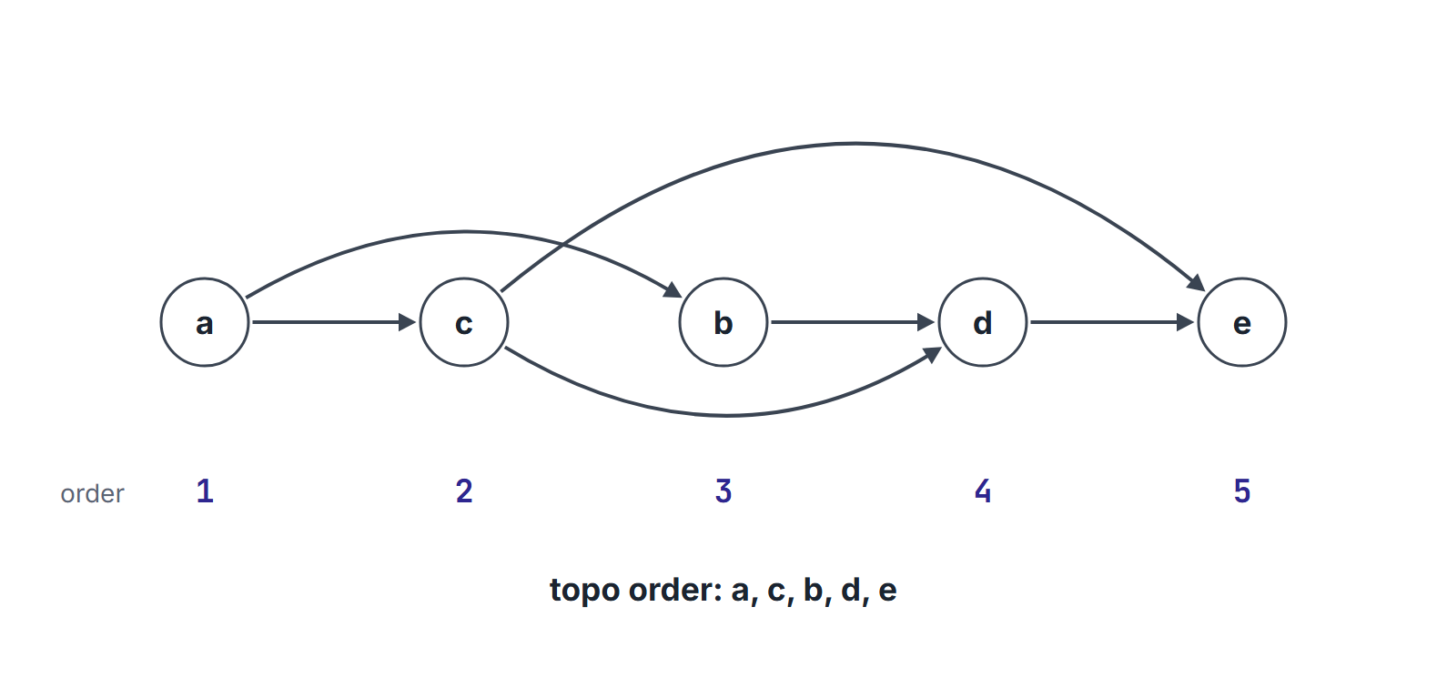
Vertices . Edges: , , , , , . One DFS (outer order ; adjacency lists alphabetical) runs as follows: discover (1), (2), (3), (4); finish (5), (6), (7); discover (8), whose edges and reach black vertices (cross edges); finish (9), (10). Discovery/finish times: , , , , . Decreasing finish: . The only other valid order is , which Kahn's algorithm with a FIFO queue produces (queue contents: ; then ; then ; then ; then ). Both respect every edge.
SCCs on five vertices
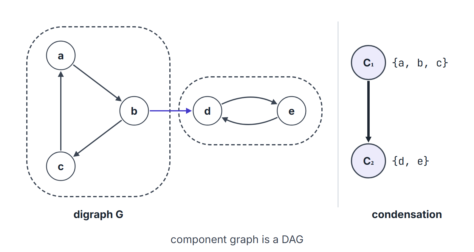
Vertices . Edges: , , , , , . SCCs: and . The component graph is .
First DFS (outer order ; lists , , , , ): discover (1), (2), (3); is a back edge; finish (4); discover (5), (6); is a back edge; finish (7), (8), (9), (10). Finish order ; decreasing finish order .
Second DFS on (edges , , , , , ) in the order : from it reaches and then , and the edge back to is already used, giving the tree . The next unvisited vertex in the order is ; its edge to leads to a visited vertex, and it reaches , giving . Here , matching the component edge .
Edge cases and implementation notes
- A zero-vertex graph has the empty topological order and no SCCs. A singleton without a self-loop has the one-vertex order and one SCC. A self-loop prevents a topological order; the vertex still belongs to an SCC.
- A complete directed cycle of vertices is one SCC and has no topological order.
- Parallel edges and self-loops: a self-loop is a back edge (cycle); parallel edges do not change reachability, but Kahn counts and decrements indegree once per edge occurrence.
- When adjacency lists are stored only for outgoing edges, building must create entries for vertices that had indegree but no outdegree in .
- Stable sorting of finish times is unnecessary: any total order that respects the numeric finish values works for Kosaraju's second pass.
Comparing the two topological algorithms in an exam answer: DFS needs recursion (or an explicit stack) and produces one valid order tied to adjacency order; Kahn's algorithm makes indegrees explicit and naturally detects cycles by counting emitted vertices. Both are .
Important properties and observations
- Topological orders are not unique when incomparable vertices exist.
- Adding an edge can merge SCCs (never split them); the number of SCCs never increases (CLRS Exercise 22.5-1). One new edge can merge many components at once: on a directed path ( singleton SCCs), adding leaves a single SCC.
- The transpose has the same SCCs as .
- A single-vertex SCC is possible even when the vertex has in- and out-edges (they leave the component).
Common misconceptions.
- "Any DFS order is a topological order." Only decreasing finish time (or Kahn's emission order) works; discovery order does not.
- "SCCs can be found by one DFS." One DFS finds trees, not SCCs; Kosaraju needs the transpose pass. Tarjan's single-pass algorithm exists but is beyond this note.
- "The second Kosaraju pass can run on ." It must run on ; on it merges components.
- "The vertex finishing last in a DAG's DFS is a sink." It is a source (it comes first in the topological order); the vertex finishing first is a sink.
- "The component graph may have cycles." By construction it is a DAG.
GATE examination perspective
- EMIT BY FINISH TIME. List vertices by decreasing .
- DETECT A CYCLE. A back edge during the topo DFS, or Kahn emitting fewer than vertices.
- NAME THE SCCs. Trace Kosaraju's two passes on a small digraph.
- CONDENSATION. Draw the component DAG after identifying SCCs.
- COMPLEXITY. Both algorithms .
- COUNT THE ORDERS. Group the vertices that are forced into positions and multiply the free interleavings, or remove sources recursively on a small DAG.
- KAHN VERSUS DFS. Kahn with a FIFO queue and DFS by decreasing finish time can output different valid orders; check every option against every edge.
Summary
Sources
- T. H. Cormen, C. E. Leiserson, R. L. Rivest, C. Stein, Introduction to Algorithms, 3rd ed., MIT Press, 2009: Chapter 22, Sections 22.4 (topological sort) and 22.5 (strongly connected components); Exercises 22.4-2 (counting paths), 22.5-1 (adding an edge) and 22.5-3 (second pass on G).