
Introduction
A network is a mesh of links and switches, and switching is the way data from one link is moved onto the next on its way to the destination. There are two fundamentally different answers. Circuit switching reserves a path and a fixed share of every link on it before any data flows, as the telephone network did. Packet switching reserves nothing: data is cut into packets, each packet is stored at every switch and forwarded when the next link is free.
Packet switching itself comes in two forms. In a datagram network (the Internet's IP layer) every packet carries the full destination address and is forwarded independently. In a virtual-circuit network a connection is set up first, the switches on the path keep state for it, and packets carry only a short circuit label.
The choice decides the delay formula, the use of capacity, the amount of state in switches, and what happens when a switch fails. The calculations are delay formulas (circuit set-up, message switching, packet pipelining, optimal packet size); the rest is comparison statements.
Prerequisites
- Layering, OSI and TCP/IP Reference Models: packets, headers and the network layer.
- Transmission delay (time to push bits onto a link of rate ) and propagation delay (time for a bit to travel distance at signal speed ).
Core concepts
Circuit switching
A circuit goes through three phases: set-up (signalling reserves a channel on every link of the path), data transfer, and teardown. On each link the reserved share is either a frequency band (FDM) or a time slot in every frame (TDM). With TDM, a link of rate divided into slots gives each circuit a rate .
Properties: guaranteed constant rate and delay once set up; no per-packet header; bits flow through switches without being stored; capacity reserved for a circuit is wasted while that circuit is silent; set-up time is paid before the first bit moves.
Message switching
The whole message is received at each switch, stored, then sent on. No reservation, no splitting. A long message occupies each link for its full transmission time, and the next link cannot start until the last bit has arrived. It is mainly a reference point for showing why packets are better.
Packet switching
The message is cut into packets of bounded size, each with a header. Every switch performs store-and-forward: it must receive the whole packet (to check it and read its header) before it starts sending it on. Because packets are small, different packets are on different links at the same moment, which is pipelining. Links are shared on demand (statistical multiplexing); when packets arrive faster than a link can send them, they wait in a queue, and a full buffer means loss.
Datagram versus virtual circuit
| Issue | Datagram (for example IP) | Virtual circuit (for example ATM, MPLS) |
|---|---|---|
| Set-up before data | None | Required |
| Address in each packet | Full destination address | Short VC identifier, local to each link |
| State in switches | None per flow (only a routing table) | One entry per VC passing through |
| Routing decision | For every packet | Once, at set-up |
| Order of arrival | May be reordered | In order along the fixed path |
| Effect of a switch failure | Packets reroute; only queued packets lost | Every VC through that switch is broken |
| Quality of service and congestion control | Hard | Easier: resources can be reserved at set-up |
Label swapping. A VC identifier has meaning only on one link. Each switch has a table mapping (incoming interface, incoming VC number) to (outgoing interface, outgoing VC number) and rewrites the label as it forwards. This keeps labels short and lets each switch choose free numbers on its own links.
| Incoming interface | Incoming VC | Outgoing interface | Outgoing VC |
|---|---|---|---|
| 1 | 12 | 3 | 22 |
| 2 | 63 | 1 | 18 |
| 3 | 7 | 2 | 17 |
A packet arriving on interface 1 with label 12 leaves on interface 3 with label 22.
Virtual circuit is different from circuit switching. A virtual circuit fixes the path but reserves nothing by default: packets are still stored and forwarded and still queue. Circuit switching reserves capacity, so there is no queueing inside the network.
How it works: the three timelines
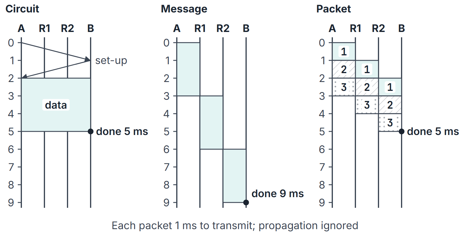
Take three links in series (host A, routers R1 and R2, host B), each of rate , with propagation delay ignored. The message is 3 packets of the same size, each needing 1 ms to transmit.
- Message switching: the whole message (3 ms of transmission) crosses each link in turn. Last bit at B at ms.
- Packet switching: packet 1 reaches B at 3 ms; packets 2 and 3 follow 1 ms apart. Last bit at B at 5 ms.
- Circuit switching: after a set-up phase (take 2 ms here), bits stream through the switches without being stored, so the 3 ms of data reaches B at ms.
Mathematical explanation
Notation: links in series (so intermediate switches), each of rate bit/s and propagation delay ; a message of bits; packets of bits each (header included), packets in all. Processing and queueing are taken as zero unless a question says otherwise.
Circuit switching. After set-up time , the message is pushed once at the circuit rate (for example for an -slot TDM link) and the bits propagate across all links:
Message switching. Each of the links carries the full message after the previous link has finished:
Packet switching (store-and-forward, pipelined). The first packet needs transmission times to reach the destination; each later packet arrives one transmission time after the one before it:
Proof sketch: with equal link rates, packet (counting from 1) finishes on link at time plus propagation, because link is busy with packet until and receives packet from link at the same moment. Set and .
Optimal packet size. The expression below assumes every packet, including the last, is padded to payload bits, so every packet has bits. An unpadded last packet requires its actual length and packet-by-packet timing. Restrict payload to the allowed integer range, normally . If a message of payload bits is cut into packets carrying payload bits plus an -bit header, then and
Small packets pipeline well but pay many headers; large packets pay few headers but pipeline badly. Ignoring the ceiling and differentiating gives an interior stationary minimum for , at
For this padded model, is a candidate/guide, not a substitute for the feasible integer search: evaluate allowed payloads (or packet-count breakpoints) and boundaries; if exceeds the maximum, test that boundary. If is feasible and is an integer, it attains the continuous lower bound. For , use one packet; for , there is no positive interior stationary minimum. An unpadded last packet requires its actual length in a packet-by-packet calculation.
Statistical multiplexing. If users each are active independently with probability , the number active is binomial, and the chance that more than are active at once is .
Worked examples
Example 1: a TDM circuit
A file of 1,000,000 bits is sent over a circuit on links of 2.048 Mbps, each divided by TDM into 32 slots; set-up takes 250 ms; propagation is ignored. Circuit rate bit/s. Transfer time s. Total s. The answer does not depend on the number of links, because the bits are not stored at switches.
Example 2: message switching against packet switching
A 1,200,000-bit message crosses 3 links of 1 Mbps, propagation ignored. Message switching: s. Packet switching with 1000 packets of 1200 bits (headers ignored): ms s. Pipelining makes the total close to one transmission of the message plus two packet times.
Example 3: optimal packet size
A 30,000-bit payload crosses links of 1 Mbps; every packet has a 100-bit header; propagation ignored. Then bits, giving 30 packets of 1100 bits and ms.
| Payload per packet (bits) | Packets | (ms) |
|---|---|---|
| 500 | 60 | 37.8 |
| 1000 | 30 | 36.3 |
| 1500 | 20 | 36.8 |
| 2000 | 15 | 37.8 |
| 30,000 (one packet) | 1 | 120.4 |
Because divides 30,000 exactly, the formula's optimum is also the best integer packet size.
Example 4: why packet switching admits more users
A 1 Mbps link; each user sends at 100 kbps while active and is active 10% of the time, independently. Circuit switching can admit 10 users. With packet switching and 40 users, the probability that more than 10 are active at once is about 0.0015, so 40 users share the link with rare overload.
Example 5: label swapping
Using the table in "Core concepts", a packet that enters on interface 3 with VC 7 leaves on interface 2 carrying VC 17. The next switch looks up (its incoming interface, 17), not 7.
Example 6: links of different rates
Three 1000-bit packets cross two links, 1 Mbps then 0.5 Mbps (1 ms and 2 ms per packet), with propagation ignored. Packet 1 reaches the router at 1 ms and the destination at 3 ms. Packet 2 reaches the router at 2 ms but waits until the slow link is free at 3 ms, so it arrives at 5 ms; packet 3 arrives at 7 ms. With all packets ready at the source, the pipelined formula becomes
one packet's time across every link plus one slowest-link time for each further packet: ms. The order of the links does not matter (slow link first also gives 7 ms), and with equal rates the formula reduces to .
Important properties and observations
- Store-and-forward is per packet, not per bit. A switch cannot start sending a packet until it has the last bit. This is why message switching multiplies the full message time by the number of links.
- Equal link rates assumed. needs equal rates. With different rates, simulate packet by packet: the slowest link sets the spacing between arrivals.
- Header overhead cuts both ways. Splitting into more packets always adds header bits; the gain comes only from pipelining, and it vanishes when (one link: one big packet is best).
- Circuit switching has no per-hop transmission term. Its delay is set-up plus one transmission at the circuit rate plus propagation.
- Virtual circuits still queue. Fixed path, in-order delivery, but no reserved capacity unless the set-up also reserves it.
Common misconceptions.
- "Packet switching is always faster." Not for one link with headers, and not against a circuit whose set-up time is negligible compared with the transfer.
- "A virtual-circuit number identifies the connection end to end." It is local to one link and is rewritten at every switch.
- "Datagram networks keep no state." Routers keep routing tables, but no per-connection state.
GATE examination perspective
- Pipelined packet delay. Count links, not routers: links means routers. Use plus propagation delays, and include the header in .
- Optimal packet size. Write , then test the candidate values given in the problem rather than trusting the square-root formula when is not an integer.
- Circuit set-up. The set-up time is added once; the TDM slot share divides the rate.
- Comparison statements. Datagram: no set-up, independent routing, reordering possible, robust to failure. VC: set-up, per-VC state, in-order, failure breaks circuits.
- Message versus packet. Message switching multiplies the full message time by the number of links.
Summary
Sources
- J. F. Kurose, K. W. Ross, Computer Networking: A Top-Down Approach, 8th ed., Pearson, 2021: Sections 1.3.1 (Packet Switching) and 1.3.2 (Circuit Switching).
- A. S. Tanenbaum, D. J. Wetherall, Computer Networks, 5th ed., Pearson, 2011: Section 2.6.5 (Switching), Sections 5.1.1 (Store-and-Forward Packet Switching), 5.1.3 and 5.1.4 (connectionless and connection-oriented service) and 5.1.5 (Comparison of Virtual-Circuit and Datagram Networks).
- B. A. Forouzan, Data Communications and Networking, 5th ed., McGraw-Hill, 2013: Chapter 8 (Switching).