
Introduction
Link and path performance is described by a few quantities: how long a packet takes to cross a link or a path (delay or latency), how many bits per second actually arrive (throughput), and how many bits are "in flight" on a path at once (the bandwidth-delay product). Efficiency formulas for stop-and-wait, sliding windows, CSMA/CD and TCP are all built from these.
Two delays that sound alike must be kept apart. Transmission delay is how long it takes to push a packet's bits onto the link; it depends on the packet size and the link rate. Propagation delay is how long one bit takes to travel the length of the link; it depends on distance and signal speed. Which one dominates decides almost every design choice in the later notes.
Prerequisites
- Circuit, Packet and Virtual-Circuit Switching: store-and-forward and pipelining of packets.
Core concepts
The four components of nodal delay
| Component | Symbol | Formula | Depends on |
|---|---|---|---|
| Processing | given | Header checks, table lookup (microseconds in routers) | |
| Queueing | from traffic | How many bits are ahead in the output buffer | |
| Transmission | Packet length (bits), link rate (bit/s) | ||
| Propagation | Link length , signal speed (about m/s in copper and fibre, m/s in free space) |
The nodal delay at one hop is .
Transmission versus propagation. has nothing to do with distance: a 1000-byte packet takes the same time to put onto a 10 m link or a 10,000 km link of the same rate. has nothing to do with packet size or link rate: a bit takes the same time to cross the link whether the link is 1 kbps or 100 Gbps.
Units convention used in all CN notes. Link rates use powers of ten: 1 kbps = , 1 Mbps = , 1 Gbps = bit/s. Sizes in bytes are multiplied by 8. Unless a question says otherwise, 1 KB = 1000 bytes; when it says , use that, because the answer changes (Example 4).
Round-trip time and the ratio
The round-trip time (RTT) is the time from sending a bit until a reply can come back; on a single link with negligible reply size and processing it is . The dimensionless ratio
compares the two delays. If (short links, long frames) the sender finishes a frame long after its first bit has arrived; if (long or fast links) the sender has finished before the first bit arrives, and the link holds many frames at once. The efficiency of stop-and-wait is and that of CSMA/CD falls as grows (Sliding Window Protocols, Medium Access Control).
Bandwidth-delay product
The bandwidth-delay product is the number of bits a link or path holds when the sender transmits continuously:
The round-trip form is the amount a sender must be allowed to have outstanding (sent but not acknowledged) to keep the link fully busy. A window smaller than caps throughput at . The physical length of one bit on the wire is metres.
Throughput
Throughput is the rate at which bits arrive at the receiver, as opposed to the link rate (often called bandwidth). For a path of links in series, the end-to-end throughput of one flow is the bottleneck rate:
where a link shared equally by flows contributes . The time to move a file of bits is about plus the path latency, and for large files the first term dominates.
Utilisation of a link is the fraction of time it is busy sending useful bits; useful throughput is utilisation times .
Traffic intensity and queueing
If packets of bits arrive at a router output at an average packets per second, the traffic intensity is . If it exceeds 1, bits arrive faster than they can leave and the queue grows without bound (in practice, packets are dropped when the buffer is full). As it approaches 1 from below, the average queueing delay grows sharply. Queueing delay is the only component that varies from packet to packet.
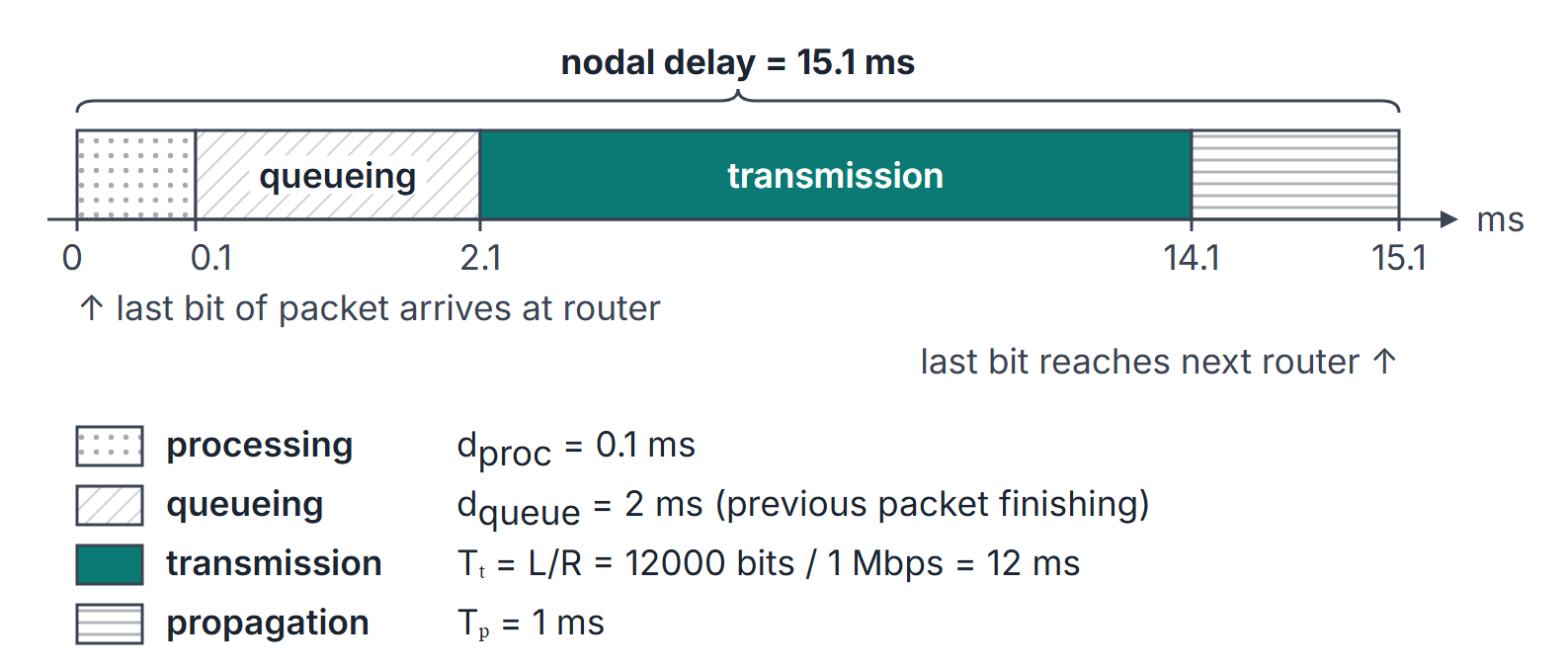
Mathematical explanation
End-to-end delay over store-and-forward links. With equal rates, no queueing and processing at each of the routers, one packet needs
and back-to-back packets need plus the propagation and processing terms (Circuit, Packet and Virtual-Circuit Switching).
Burst queueing. If packets of bits arrive at an idle link at the same instant, the -th one (counting from 1) waits , so the average queueing delay is
Window-limited throughput. A sender allowed at most bits outstanding sends bits per RTT at best, so
Worked examples
Example 1: which delay dominates
A 1000-byte packet (8000 bits) on a 10 Mbps link, signal speed m/s.
| Link length | Dominant | |||
|---|---|---|---|---|
| 2000 km | 0.8 ms | 10 ms | 12.5 | Propagation |
| 100 m | 0.8 ms | 0.5 µs | 0.000625 | Transmission |
On a 1 Gbps link 3000 km long, a 1 MB file (8,000,000 bits) has ms and ms: even a large transfer is propagation-dominated on a fast long-haul link.
Example 2: end-to-end delay over three links
Host to host through two routers: three links of 1 Mbps, each with ms, packets of 1500 bytes (12,000 bits, so ms), no queueing.
- One packet, no processing: ms.
- One packet, 0.1 ms processing at each router: 39.2 ms.
- Ten back-to-back packets, no processing: ms.
Example 3: bandwidth-delay product
A 100 Mbps path with RTT 40 ms: bits bytes must be outstanding to keep it busy. One way (20 ms) the path holds bits. At m/s each bit is m long.
A geostationary satellite link with ms each way (RTT 540 ms) at 10 Mbps has a round-trip BDP of bits bytes. A sender limited to a 65,535-byte window gets at most bit/s, under 1 Mbps on a 10 Mbps link. This is why TCP needs window scaling on such paths (TCP Flow Control).
Example 4: bottleneck throughput and the KB trap
A server with a 2 Mbps access link sends to a client with a 1 Mbps access link through a 50 Mbps core link shared equally by 10 flows (5 Mbps each). Throughput is Mbps. A 4 MB file takes s with 1 MB = bytes, but s with 1 MB = bytes.
Example 5: traffic intensity
Packets of 12,000 bits arrive at 100 packets/s at a 1.5 Mbps link: . At 150 packets/s the intensity is 1.2, and the queue grows without bound until the buffer overflows.
Example 6: a burst
Five 12,000-bit packets arrive together at an idle 1 Mbps link. Their queueing delays are 0, 12, 24, 36 and 48 ms; the average is 24 ms, which matches .
Important properties and observations
- Latency versus throughput. Short transfers (a DNS query, a TCP handshake) are limited by RTT; long transfers are limited by the bottleneck rate or the window. Doubling the link rate halves but leaves alone.
- BDP sets the window. Any protocol that waits for acknowledgements needs a window of at least (in bits or the matching number of frames) to reach full utilisation.
- Processing and queueing. Use them only when a problem gives them; otherwise take them as zero.
- Bits versus bytes. A missing factor of 8, or mixed with , changes the answer; keep the units written out.
Common misconceptions.
- "A faster link reduces propagation delay." It does not; only distance and medium matter.
- "Bandwidth is throughput." Bandwidth (link rate) is the maximum; throughput is what a flow actually gets, at most the bottleneck.
- "RTT is twice the one-way delay of the data packet." RTT is usually defined by propagation (plus small reply times); the transmission time of the data frame is added separately in efficiency formulas.
GATE examination perspective
- Definition of . . Some books write efficiency formulas with defined as round-trip over transmission; read the formula's derivation, not its letters.
- Which delay dominates. Compare with numerically.
- Store-and-forward chains. links means transmission times and propagation delays for one packet.
- BDP calculations. "How many bits are on the link" is ; "how large must the window be" is (often plus one frame time, as in sliding-window efficiency).
- Unit traps. KB as 1000 or 1024, bits versus bytes, ms versus µs.
Summary
Sources
- J. F. Kurose, K. W. Ross, Computer Networking: A Top-Down Approach, 8th ed., Pearson, 2021: Section 1.4 (1.4.1 Overview of Delay in Packet-Switched Networks, 1.4.2 Queuing Delay and Packet Loss, 1.4.3 End-to-End Delay, 1.4.4 Throughput in Computer Networks).
- A. S. Tanenbaum, D. J. Wetherall, Computer Networks, 5th ed., Pearson, 2011: Section 6.6.6 (Protocols for Long Fat Networks), for the bandwidth-delay product and window limits.
- D. Borman, B. Braden, V. Jacobson, R. Scheffenegger (Ed.), RFC 7323, TCP Extensions for High Performance, 2014, Section 1.1 (TCP Performance: the bandwidth-delay product and the window size limit of the 16-bit window field), (consulted 2026-11-11).