
Introduction
A table, bar chart, pie chart, line graph, scatter plot or map-like grid displays numbers. A value is then read from the display, or computed from the values read: a growth rate, a share, a ratio, an average, or the category that satisfies a condition. The arithmetic is that of Ratios and Percentages; the skill specific to DI is reading the display correctly and choosing the right base for each percentage.
Every chart type has its own reading rule (a bar is read at its top against the axis, a pie slice is a share of 360 degrees, a line's slope is a rate of change), and its own trap. The material is a reading procedure, the formulas for the common derived quantities, and one data set shown in three charts, worked through question by question, plus a scatter plot.
Prerequisites
- Ratios and Percentages: percentage change, shares, ratios, percentage points.
- Averages: mean and median of a short list (Elementary Statistics and Probability, linked under Related topics).
Core concepts
| Display | What it encodes | Reading rule | Typical trap |
|---|---|---|---|
| Table | Exact values by row and column | Read the units and the row and column headings | Totals row or column included or not |
| Bar chart | Value as bar length | Read the top of the bar against the axis | Axis not starting at 0 exaggerates differences |
| Stacked bar | Parts and their total | A segment's value is its top minus its bottom | Reading a segment's top as its value |
| Pie chart | Share of a whole | Share angle | Comparing slices of two pies with different totals |
| Line graph | Value over an ordered axis | Slope is change per unit of the horizontal variable | For equal horizontal intervals, steeper magnitude means larger absolute change, not necessarily larger percentage growth |
| Scatter plot | Two variables per item | Each point is ; a line through the origin with slope marks | Points exactly on a boundary line |
| 3-D or perspective chart | Same as its 2-D form | Read the front face of a bar or the labelled value, not the drawn depth | Depth makes rear bars look taller |
| Map or grid | Values by location | Read the legend and scale first | Colour bands are ranges, not exact values |
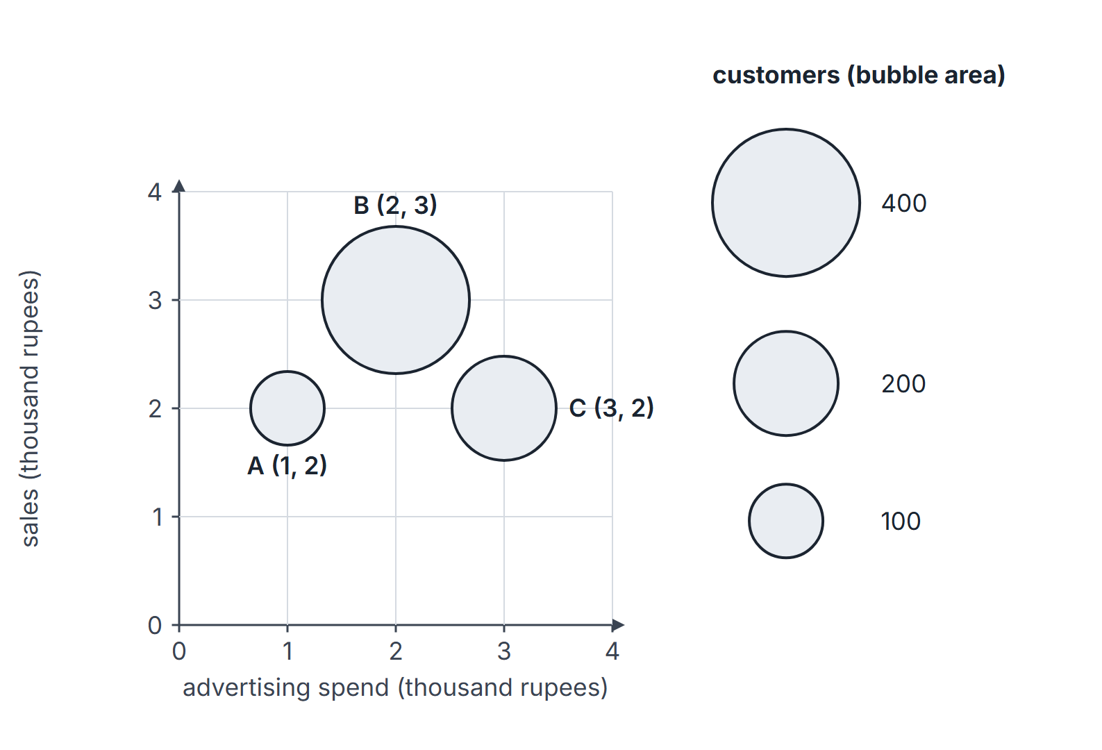
A 3-D surface plot shows a third variable as height above an - grid (often also colour-coded); a bubble chart shows it as bubble size (by convention, area). Read the third value from the labelled vertical axis, contour labels or legend, not from apparent height or size in a perspective drawing.
Derived quantities.
- Percentage change from to : .
- Share of a part in a total : ; its pie angle is .
- Average over periods: total .
- Compound average growth over steps from to : (see Powers, Exponents and Logarithms).
Rounding convention. Worked percentages are rounded to two decimal places at the last step; intermediate values are kept exact.
A data set in three displays
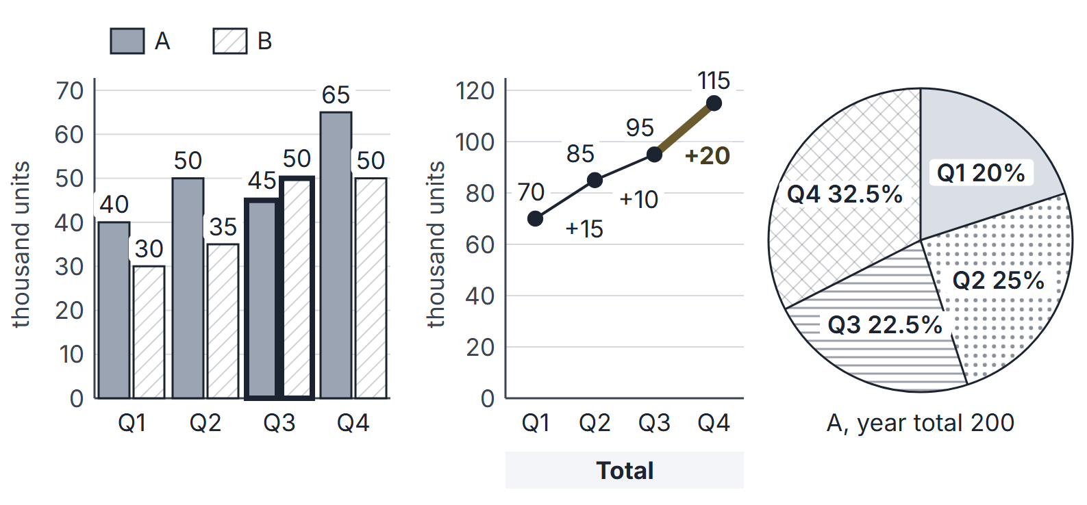
A factory makes two products, A and B. Production in thousand units per quarter:
| Quarter | A | B | Total |
|---|---|---|---|
| Q1 | 40 | 30 | 70 |
| Q2 | 50 | 35 | 85 |
| Q3 | 45 | 50 | 95 |
| Q4 | 65 | 50 | 115 |
| Year | 200 | 165 | 365 |
Reading procedure
- Read the frame first. Title, units (thousands, lakhs, percent), axis labels and scale, legend, and whether the axis starts at 0.
- Restate the question as a formula before reading any value: "percentage increase of total from Q1 to Q4" is .
- Read only the values needed, and write them down with units.
- Approximate first to eliminate options; compute exactly only if two options are close.
- Check the base of every percentage and whether the question asks for percent or percentage points.
- For "how many" or "which" questions, test every category against the condition, including the boundary cases.
Worked examples on the production data
Example 1 (growth). Percentage increase in total production from Q1 to Q4: .
Example 2 (largest step). Quarter-on-quarter increases in the total are , and . The largest increase is into Q4. On the line graph this is the steepest segment.
Example 3 (ratio). Ratio of A to B in Q3: .
Example 4 (average). Average quarterly production of B: thousand units.
Example 5 (share and pie angle). A's annual production by quarter as shares of 200: Q1 , Q2 , Q3 , Q4 . The pie angles are these shares of : , , , , which sum to .
Example 6 (condition test). In which quarters did B produce more than A? Only Q3 (50 against 45). In Q4 B equals its Q3 value but A rose to 65.
Example 7 (percent versus percentage points). A's share of the quarterly total was in Q1 and in Q4. The share fell by about percentage points, even though A's own production rose by .
Example 8 (comparing across displays). "B's Q3 bar is taller than A's Q3 bar" and "A's Q3 slice is smaller than its Q4 slice" are both true, but a pie of B's production (total 165) could not be compared slice by slice with this pie of A's (total 200): equal angles in the two pies would mean equal shares, not equal quantities.
Example 9 (compound average growth). Total production rose from 70 to 115 over three quarter-steps. The compound growth rate per quarter is , while the simple average of the three step rates , , is about . They are close here but not equal in general.
A scatter plot
Six shops U, V, W, X, Y, Z report advertising spend and sales , both in lakh rupees: U , V , W , X , Y , Z .
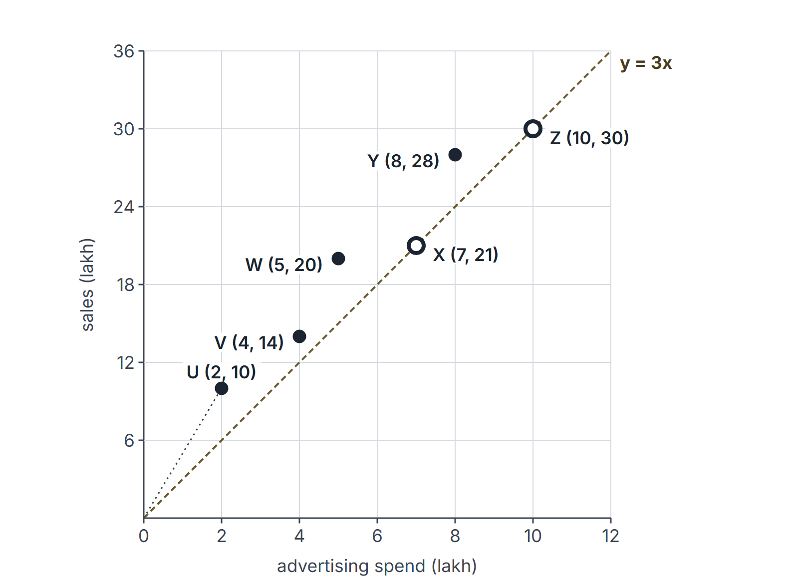
Example 10 (ratio from a scatter plot). Sales per lakh of spend: U 5, V 3.5, W 4, X 3, Y 3.5, Z 3. The highest is U. On the plot, U is the point whose line to the origin is steepest.
Example 11 (boundary trap). How many shops have sales more than three times their spend? U, V, W and Y: 4 shops. X and Z have exactly three times and do not count. A question saying "at least three times" would give 6.
Example 12 (centre). Mean sales: lakh. Median spend: the spends sorted are 2, 4, 5, 7, 8, 10, so the median is lakh.
Shares, totals and growth rates
Example 13 (ratio of percentage-of-whole values). A company's expenses were 800 lakh in 2023 and 1,000 lakh in 2024. Two pie charts show salaries as 25% of the 2023 total and 22% of the 2024 total.
- Salary values: and lakh.
- Ratio of the values: . The ratio of the percentages, , is the wrong answer because the totals differ.
- Salaries rose by even though their share fell by 3 percentage points.
Example 14 (percent of a percent). In a firm, 40% of employees are women. 25% of the women and 15% of the men are engineers. Take 100 employees: 40 women and 60 men; engineers . So 19% of employees are engineers, and women are of the engineers. Averaging 25% and 15% to get 20% ignores the unequal group sizes.
Example 15 (CAGR versus average growth). Revenue went 1,000, then 1,200, then 1,080, then 1,331 over three years.
- Yearly growth rates: , , and . Their simple average is about .
- Compound annual growth rate (CAGR): .
- Only the CAGR reproduces the end value: . Growing at 11.08% each year would give about 1,371.
Example 16 (when the gap is large). A value goes from 100 to 200 and back to 100. The yearly rates are and ; their average is , but the CAGR is , since the value ended where it started. The simple average of rates overstates growth whenever rates vary.
Example 17 (map or table of regions). A district map is divided into four labelled regions, with population (thousands) and area (square kilometres) given in a table printed on the map:
| Region | North | East | South | West |
|---|---|---|---|---|
| Population | 40 | 30 | 20 | 15 |
| Area | 8 | 5 | 10 | 5 |
Density is population divided by area. East has density , North , West and South , so East is the densest. East's share of the total population is . A colour band on a choropleth map would only place East in a range such as "5 to 7"; the table on the map is what gives the exact values.
Three-variable worked example. A bubble plot uses horizontal = advertising spend (thousand rupees), vertical = sales (thousand rupees), and bubble area = customers . Plot A at with , B at with , and C at with . The legend's 100-customer bubble has radius 1 plotting unit of size, so B has radius 2 and C radius ; positions use the axis scales independently of this size scale. B represents 400 customers versus A's 100: four times the area, but only twice the radius. C represents 200 customers, twice A's count. Do not read from the y-coordinate or apparent perspective height.
Important properties and observations
- Absolute versus relative. The largest absolute increase need not be the largest percentage increase: the Q1 to Q2 step of 15 is , the Q3 to Q4 step of 20 is .
- Shares of different totals. A share can fall while the quantity rises (Example 7); a pie compares only within itself (Example 8).
- Truncated axes. When a bar chart's axis starts above 0, bar heights are not proportional to values; compute from the axis labels.
- Stacked bars. Only the bottom segment can be read directly against the axis; every other segment is a difference.
- Common misconceptions. "The steepest line segment has the largest percentage growth" (it has the largest absolute growth for equal steps). "Equal pie angles mean equal amounts" (only within one pie).
- EDGE CASE. Growth from a value of 0 has no percentage; report the absolute change.
GATE examination perspective
- Base traps. Percentage change is on the earlier value; share is on the total of the stated group (Examples 1 and 5).
- Percentage-point traps. A change of share is in percentage points (Example 7).
- Boundary traps. "More than", "at least" and "exactly" give different counts (Example 11).
- Cross-display traps. Combining two pies or a pie and a bar chart needs the actual totals (Example 8).
- Estimation. When the options are far enough apart, a two-significant-figure estimate decides; keep exact arithmetic for close options.
- Units. Values in thousands or lakhs must be scaled when the answer asks for units.
- Shares across different totals. Convert each percentage to a value before comparing; a falling share can hide a rising value (Example 13).
- Percent of a percent. Work with a base of 100 and count; do not average percentages of unequal groups (Example 14).
- CAGR versus average growth. The CAGR is the rate that reproduces the end value; the simple average of yearly rates is larger whenever the rates vary (Examples 9, 15 and 16).
Summary
Sources
- B. Illowsky, S. Dean et al., Introductory Statistics 2e, OpenStax, 2023: Section 2.1 Stem-and-Leaf Graphs (Stemplots), Line Graphs, and Bar Graphs; Section 2.2 Histograms, Frequency Polygons, and Time Series Graphs. (consulted 2026-11-11).
- D. Kirk et al., Contemporary Mathematics, OpenStax, 2023: Section 8.2 Visualizing Data; Section 8.8 Scatter Plots, Correlation, and Regression Lines. (consulted 2026-11-11).
- GATE 2027 General Aptitude syllabus, IIT Madras, Section 2 "Data interpretation: data graphs (bar graphs, pie charts, and other graphs representing data), 2- and 3-dimensional plots, maps, and tables". (consulted 2026-11-11).