
Introduction
Interactive systems care about response time: a user who presses a key wants a reaction now, not after a long batch job finishes. Round robin (RR) achieves this by time slicing. Every ready process gets the CPU for at most one time quantum , then goes to the back of the queue. Among ready processes, no process waits more than quanta for its next turn.
Real systems mix interactive and batch work, so they use several ready queues with different policies. A multilevel queue assigns each process permanently to one queue; a multilevel feedback queue (MLFQ) moves processes between queues according to how they behave, so that short and interactive jobs float to the top without the scheduler knowing burst lengths in advance.
The same four-process workload as CPU Scheduling: Criteria, FCFS, SJF, SRTF and Priority is used, so the results can be compared directly.
Prerequisites
- CPU Scheduling: Criteria, FCFS, SJF, SRTF and Priority: turnaround, waiting and response time; the tie conventions; preemption.
Core concepts
Round robin
- The ready queue is FIFO. The dispatcher takes the head, sets the timer to and runs it.
- If the burst finishes within , the process leaves and the next one starts at once.
- If the timer expires, the process is preempted and appended to the tail.
- A process never gets more than consecutive units while others are ready. (If it is the only ready process, it simply gets another quantum.)
Queue-order convention used in the traces. When a process arrives at the same instant that the running process's quantum expires, the new arrival joins the queue first and the preempted process goes behind it. A stated problem may use the opposite order; follow the problem.
Quantum size.
| Quantum | Behaviour |
|---|---|
| larger than every burst | Identical to FCFS |
| very small | Approaches processor sharing (each of processes runs at speed ); context-switch overhead dominates |
| Rule of thumb | Most CPU bursts (often quoted as about 80%) should finish within one quantum |
Waiting bound. With processes in the ready queue and switch time , the gap between the end of one quantum of a process and the start of its next is at most : the other processes run once each, and there are switches (one before each of their runs and one back). With free switching this is the familiar .
Multilevel queue
The ready queue is split into separate queues, for example system, interactive and batch processes. Each process is placed in one queue for life, and each queue has its own algorithm (RR for interactive, FCFS for batch). Scheduling between queues is either:
- Fixed priority: a lower queue runs only when all higher queues are empty. A higher-queue arrival preempts a lower-queue process. Lower queues can starve.
- Time slicing: each queue gets a share of CPU time, for example 80% to the foreground and 20% to the background.
Multilevel feedback queue
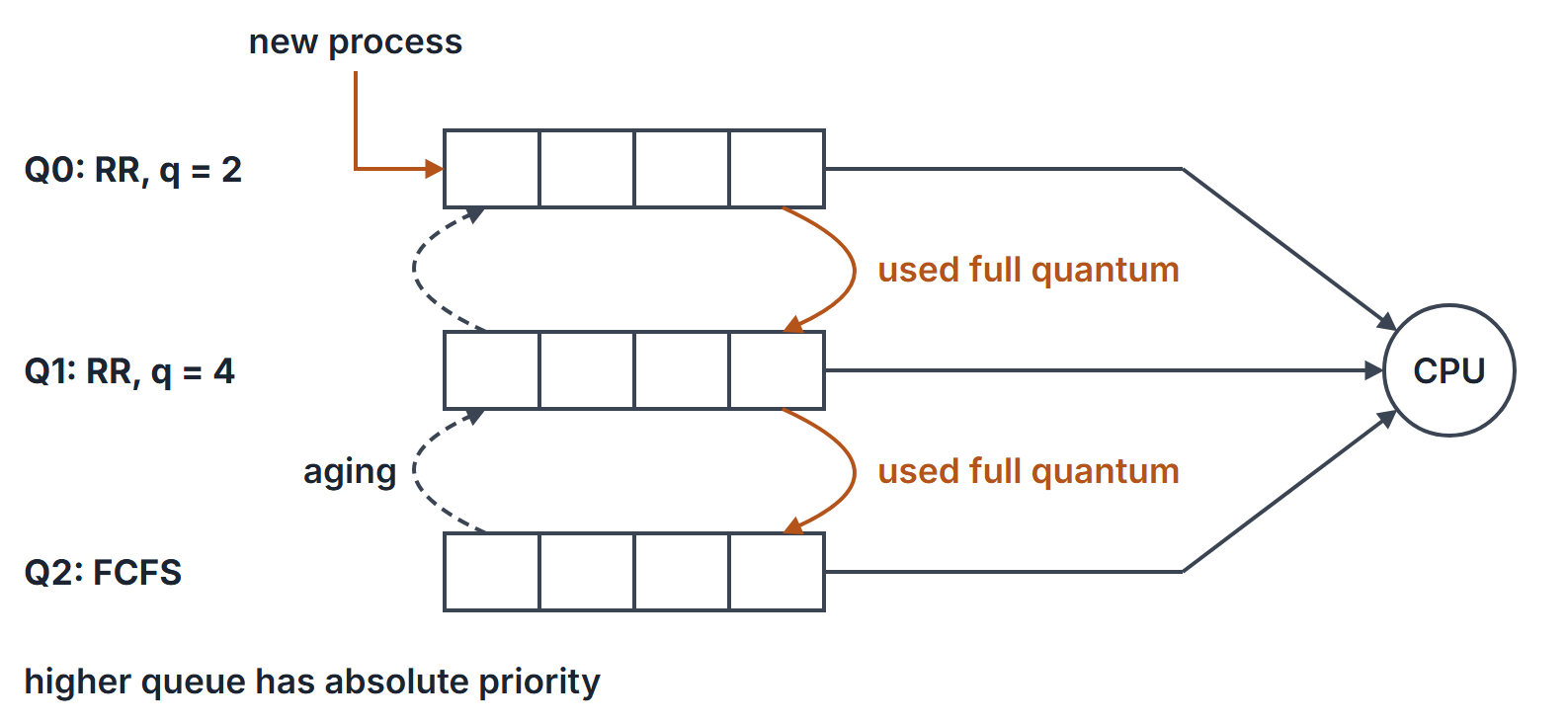
Processes move between queues. A typical configuration:
- Q0: RR with ; Q1: RR with ; Q2: FCFS.
- Every new process enters Q0.
- A process that uses its whole quantum is demoted one level (it looks CPU-bound).
- A process that blocks or finishes before its quantum ends stays at its level.
- A higher queue has absolute priority. An arrival in Q0 preempts a process running from a lower queue; the preempted process returns to the tail of its own queue with a fresh quantum.
- Aging: a process that waits too long in a low queue is promoted, which prevents starvation.
An MLFQ is defined by: the number of queues, the algorithm and quantum of each, the demotion rule, the promotion (aging) rule, and the entry queue for new processes. A problem must give these explicitly; the traces use the rules just stated.
Mathematical explanation
Response time bound. In RR with ready processes, between two consecutive quanta of one process every other process runs at most once, for at most , with one switch before each run and one more switch back to the process. So the gap is at most . Example: , , gives units.
Overhead. If every quantum is used in full, the useful fraction of CPU time is . With and , that is 80%, matching the example.
Number of quanta. A burst of length needs quanta in RR, so it is preempted times (assuming other processes are always ready).
Worked examples
The workload (from the previous note, priorities not used):
| Process | Arrival | Burst |
|---|---|---|
| P1 | 0 | 7 |
| P2 | 2 | 4 |
| P3 | 4 | 1 |
| P4 | 5 | 4 |
Round robin with
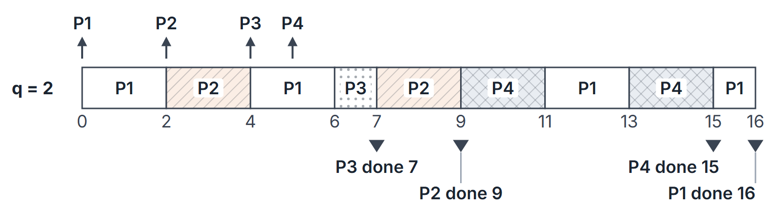
Trace of the ready queue (head on the left):
| Time | Event | Queue after the event |
|---|---|---|
| 0 | P1 arrives and runs | (empty) |
| 2 | P2 arrives; P1's quantum expires; arrival first | P2, P1 |
| 2 | P2 runs | P1 |
| 4 | P3 arrives; P2 expires (2 left) | P1, P3, P2 |
| 4 | P1 runs | P3, P2 |
| 5 | P4 arrives | P3, P2, P4 |
| 6 | P1 expires (3 left); P3 runs | P2, P4, P1 |
| 7 | P3 finishes; P2 runs | P4, P1 |
| 9 | P2 finishes; P4 runs | P1 |
| 11 | P4 expires (2 left); P1 runs | P4 |
| 13 | P1 expires (1 left); P4 runs | P1 |
| 15 | P4 finishes; P1 runs | (empty) |
| 16 | P1 finishes |
Gantt: P1 0 to 2, P2 2 to 4, P1 4 to 6, P3 6 to 7, P2 7 to 9, P4 9 to 11, P1 11 to 13, P4 13 to 15, P1 15 to 16.
| Process | CT | TAT | WT | RT |
|---|---|---|---|---|
| P1 | 16 | 16 | 9 | 0 |
| P2 | 9 | 7 | 3 | 0 |
| P3 | 7 | 3 | 2 | 2 |
| P4 | 15 | 10 | 6 | 4 |
Average WT , average TAT , average RT . Compare FCFS: average RT 4.75. Round robin gives up some waiting time to gain response time.
Effect of the quantum
| Average WT | Context switches between different processes | |
|---|---|---|
| 1 | 5.5 | 14 |
| 2 | 5 | 8 |
| 3 | 7 | 7 |
| 4 | 4.5 | 4 |
| 7 | 4.75 (same schedule as FCFS) | 3 |
Average waiting time is not monotonic in . It rose from to and fell again at . Smaller quanta generally tend to increase switching overhead, but the switch count is not a monotonic law for every workload. Exact counts require the arrivals, bursts, tie rules and switch-counting convention; for the displayed workload and model, use the counts in the table.
Adding switch cost
If each of the 8 switches at costs 1 unit, the last process finishes at and CPU utilization falls to . With the same cost gives and utilization .
Quantum edge cases
Arrival at the instant a quantum expires. P1 (arrival 0, burst 4), P2 (1, 3), P3 (2, 2), . At time 2, P1's quantum expires and P3 arrives.
| Rule at time 2 | Gantt chart | CT of P1, P2, P3 | WT of P1, P2, P3 |
|---|---|---|---|
| New arrival first (the convention used in the traces) | P1 0 to 2, P2 2 to 4, P3 4 to 6, P1 6 to 8, P2 8 to 9 | 8, 9, 6 | 4, 5, 2 |
| Preempted process first | P1 0 to 2, P2 2 to 4, P1 4 to 6, P3 6 to 8, P2 8 to 9 | 6, 9, 8 | 2, 5, 4 |
Both give an average WT of , but individual completion times differ, so a question that asks about one process depends on the rule. P2 arrived at 1, before the quantum expired, so it is ahead of both under either rule.
A burst that ends exactly at the quantum. In the chart above, P1's second run uses its remaining 2 units, exactly one quantum. The process terminates; it is not put back in the queue, and no extra switch is counted for it.
A lone process. If only one process is ready when its quantum expires, it continues; whether that counts as a context switch is a convention. Only switches between different processes are counted, so a lone process that continues is not a switch, since no other process's state is loaded; read the question's rule.
Largest quantum for a response limit. Five processes are always ready, , and each process must wait at most 30 units between the end of one of its quanta and the start of its next. The bound gives , so and the largest integer quantum is 6, with a gap of exactly 29. A simulation with and measures gaps of 29 and 33.
A multilevel feedback queue trace
Q0 (RR, ), Q1 (RR, ), Q2 (FCFS), with the rules above. Jobs: A (arrival 0, burst 9), B (1, 3), C (2, 1).
- 0 to 2: A runs in Q0 and uses its full quantum: demoted to Q1. At 2, C arrives into Q0 behind B.
- 2 to 4: B runs in Q0, full quantum, 1 left: demoted to Q1 (behind A).
- 4 to 5: C runs in Q0 and finishes.
- 5 to 9: A runs in Q1 for its full quantum of 4, 3 left: demoted to Q2.
- 9 to 10: B runs in Q1 and finishes.
- 10 to 13: A runs in Q2 (FCFS) and finishes.
Completion: A 13, B 10, C 5. Waiting: A 4, B 6, C 2. The short job C finishes first even though it arrived last, without the scheduler knowing any burst length.
Preemption across levels. Change C to arrive at 6 with burst 2. Then A runs 0 to 2 (to Q1), B 2 to 4 (to Q1), and A starts its Q1 quantum at 4. At 6, C arrives in Q0 and preempts A, which goes back to the tail of Q1 with 5 units left. C runs 6 to 8, B finishes 8 to 9, and A runs 9 to 13 in a fresh Q1 quantum. It uses all 4 units with 1 still left, so it is demoted to Q2 and finishes there, 13 to 14.
Important properties and observations
- RR never starves a process; FCFS order is preserved within the queue.
- RR is preemptive by construction, even when no new process arrives.
- Average turnaround of RR is often worse than SJF; its advantage is response time and fairness.
- Fixed-priority multilevel queues can starve the low queues; MLFQ uses aging to prevent that.
- MLFQ approximates SJF: short and I/O-bound jobs stay in the top queues, CPU-bound jobs sink.
Common misconceptions.
- "A smaller quantum always reduces waiting time." The table above shows otherwise, and overhead grows.
- "In RR a finishing process wastes the rest of its quantum." The next process starts immediately.
- "Multilevel queue and multilevel feedback queue are the same." Only the feedback version moves processes between queues.
GATE examination perspective
- RR traces. Write the queue after every event and apply the arrival-before-preempted rule (or the stated rule). Queue order at a simultaneous arrival is the step that needs most care.
- Quantum extremes. the largest burst gives FCFS; tiny gives high overhead.
- Counting context switches. Count changes of running process; read whether the first dispatch and switches to idle are counted.
- Response time questions. RR bounds the gap between turns by (count the switches carefully); the largest that keeps response under a given limit follows from that bound.
- MLFQ. Track each job's level and remaining time; apply demotion only when the full quantum is used; check whether higher-level arrivals preempt.
- Starvation. Fixed-priority multilevel queues starve; RR and MLFQ with aging do not.
Summary
Sources
- A. Silberschatz, P. B. Galvin, G. Gagne, Operating System Concepts, 10th ed., Wiley: Chapter 5, Section 5.3 Scheduling Algorithms (round robin, multilevel queue, multilevel feedback queue).
- A. S. Tanenbaum, H. Bos, Modern Operating Systems, 4th ed., Pearson: Section 2.4.3 Scheduling in Interactive Systems (round robin, priority scheduling, multiple queues).