
Introduction
When several processes are ready and there is one CPU, the short-term scheduler decides which runs next. The decision is made over and over, every few milliseconds, so the policy shapes how long jobs take, how responsive the system feels and whether some process can be postponed forever.
Processes alternate between CPU bursts and I/O bursts. Scheduling is about CPU bursts: each scheduling algorithm takes the set of ready processes, each with an arrival time and a burst length, and builds a Gantt chart, a timeline showing who runs when. The chart gives completion, turnaround, waiting and response times.
The scheduling criteria and the preemption rule are used with the algorithms that choose by arrival order, by burst length and by priority: FCFS, SJF, SRTF, HRRN and priority scheduling, with the tie-breaking rules that make the schedule unique. Round robin and multilevel queues follow in Round Robin and Multilevel Queue Scheduling.
Prerequisites
- Processes, PCB and Process States: ready and waiting states, context switch, dispatch.
- A FIFO queue: the ready queue of FCFS is one (see Related topics).
Core concepts
Times and criteria
For a process with arrival time , burst time , first time on the CPU and completion time :
| Quantity | Definition |
|---|---|
| Turnaround time (TAT) | |
| Waiting time (WT) | : total time spent in the ready queue |
| Response time (RT) | : time until the first run |
| Throughput | Processes completed per unit time |
| CPU utilization | Fraction of time the CPU does useful work |
Waiting time is time in the ready queue only. For a process that also does I/O, waiting time excludes the I/O; in these CPU-burst exercises every process has one burst, so holds exactly. For a non-preemptive algorithm, response time equals waiting time, because a process never waits again once started.
Optimization goals. Maximize utilization and throughput; minimize turnaround, waiting and response time. No algorithm is best on all of them at once.
When the scheduler runs
Scheduling decisions happen when a process (1) switches from running to waiting, (2) switches from running to ready (for example, after a timer interrupt), (3) switches from waiting to ready, or (4) terminates. Non-preemptive scheduling decides only at (1) and (4): a running process keeps the CPU until it blocks or finishes. Preemptive scheduling also decides at (2) and (3): an arrival can take the CPU away from the running process.
The dispatcher performs the switch; its delay is the dispatch latency (the context-switch cost).
Tie-breaking conventions used in the traces
Tie convention used in the traces. (a) When two ready processes are equal on the algorithm's key, the one that arrived earlier goes first; if they also arrived together, the lower process number goes first. (b) In a preemptive algorithm, a newly arrived process preempts the running one only if it is strictly better; on a tie the running process keeps the CPU. (c) Priority numbers: a smaller number means higher priority. (d) Unless a question gives a context-switch cost, switching is free. A stated problem may give different rules; when it does, those rules win.
The algorithms
First-come, first-served (FCFS)
Run processes in arrival order; non-preemptive. A FIFO queue implements it.
- Simple, no starvation.
- Convoy effect: one long CPU-bound process holds the CPU while many short or I/O-bound ones wait behind it, so both the CPU and the devices are poorly used. Three jobs arriving at time 0 with bursts 20, 2, 2 in that order wait , average 14; in the order 2, 2, 20 they wait , average 2.
Shortest job first (SJF), non-preemptive
When the CPU is free, pick the ready process with the shortest burst.
- Optimal for average waiting time among non-preemptive schedules of a fixed set of jobs available together (exchange argument, section "Mathematical explanation").
- Needs burst lengths in advance, so real systems predict them.
- Starvation: a long job can wait forever if short jobs keep arriving.
Shortest remaining time first (SRTF), preemptive SJF
At every arrival, compare the new process's burst with the remaining time of the running process; switch if the new one is strictly shorter.
- Minimizes average waiting time among all schedules when arrivals are known, at the cost of more context switches.
- Same starvation risk as SJF, stronger.
Priority scheduling
Each process has a priority; the highest priority runs. Non-preemptive priority waits for the CPU to be free; preemptive priority lets a higher-priority arrival preempt. SJF is priority scheduling with priority = predicted burst.
- Starvation (indefinite blocking) of low-priority processes. The fix is aging: raise a process's priority the longer it waits.
Highest response ratio next (HRRN)
Non-preemptive. When the CPU is free, compute for each ready process
where is the time it has waited so far, and run the one with the largest . All jobs start at ratio 1. For equal positive waiting time, shorter jobs have a higher ratio and their ratio grows faster per unit waiting. This balances short-job preference with aging; starvation claims require assumptions about the workload, such as a finite set of finite jobs.
Mathematical explanation
Why SJF minimizes average waiting time
Take jobs all available at time 0, run in some order with bursts . Job waits , so the total waiting time is
The burst in position is counted times, so to minimize the sum the largest coefficients must multiply the smallest bursts: sort in increasing order. If two adjacent jobs are out of order (), swapping them changes the total by . This exchange argument proves optimality for simultaneous arrivals; with staggered arrivals the preemptive SRTF is the optimal one.
Predicting the next burst: exponential averaging
With the measured length of the -th burst and its prediction,
ignores the measured bursts (the prediction stays ); uses only the last burst. Unrolling, the weight of is : older bursts count geometrically less. Example with , and bursts 6, 4, 6: , , .
Worked examples: one workload, five algorithms
| Process | Arrival | Burst | Priority |
|---|---|---|---|
| P1 | 0 | 7 | 3 |
| P2 | 2 | 4 | 1 |
| P3 | 4 | 1 | 4 |
| P4 | 5 | 4 | 2 |
FCFS
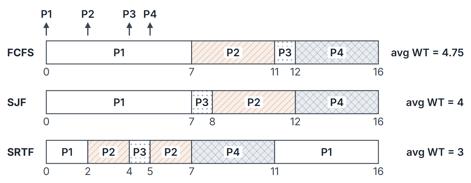
Gantt: P1 0 to 7, P2 7 to 11, P3 11 to 12, P4 12 to 16.
| Process | CT | TAT | WT |
|---|---|---|---|
| P1 | 7 | 7 | 0 |
| P2 | 11 | 9 | 5 |
| P3 | 12 | 8 | 7 |
| P4 | 16 | 11 | 7 |
Average WT ; average TAT .
SJF (non-preemptive)
At 7, P1 finishes and P2 (4), P3 (1) and P4 (4) are ready: P3 runs. At 8, P2 and P4 tie at 4; P2 arrived first. Gantt: P1 0 to 7, P3 7 to 8, P2 8 to 12, P4 12 to 16. WT: P1 0, P2 6, P3 3, P4 7; average 4. Average TAT 8.
SRTF
- At 2, P2 arrives with 4 against P1's remaining 5: P2 preempts.
- At 4, P3 arrives with 1 against P2's remaining 2: P3 preempts.
- At 5, P3 is done; P2 (2 left) beats P4 (4) and P1 (5).
- At 7, P4 (4) beats P1 (5).
Gantt: P1 0 to 2, P2 2 to 4, P3 4 to 5, P2 5 to 7, P4 7 to 11, P1 11 to 16.
| Process | CT | TAT | WT | RT |
|---|---|---|---|---|
| P1 | 16 | 16 | 9 | 0 |
| P2 | 7 | 5 | 1 | 0 |
| P3 | 5 | 1 | 0 | 0 |
| P4 | 11 | 6 | 2 | 2 |
Average WT , average TAT , average RT . SRTF beats SJF (4) on average waiting time, as it must.
Priority, non-preemptive and preemptive
Non-preemptive: P1 runs 0 to 7. At 7 the ready set is P2 (priority 1), P3 (4) and P4 (2): P2 runs 7 to 11, then P4 11 to 15, then P3 15 to 16. WT: P1 0, P2 5, P3 11, P4 6; average 5.5.
Preemptive: at 2, P2 (priority 1) preempts P1 (3) and runs to 6. At 6 the best is P4 (2), which runs 6 to 10. Then P1 (3) runs 10 to 15 and P3 (4) runs last, 15 to 16. WT: P1 8, P2 0, P3 11, P4 1; average 5. P3 has the worst waiting time in both: low priority means it waits behind everyone.
HRRN versus SJF
Jobs A (arrival 0, burst 10), B (1, 4) and C (9, 1). A runs 0 to 10. At 10, B has waited 9: ; C has waited 1: . HRRN runs B (10 to 14) then C (14 to 15). SJF would run C first (10 to 11) and then B (11 to 15). SJF has the lower average waiting time ( against ), but HRRN rewards B for having waited.
A tie in SRTF
P1 (arrival 0, burst 4) and P2 (arrival 1, burst 3). At time 1, P1 has 3 units left and P2 needs 3: a tie. Under the convention above the running P1 continues: P1 0 to 4, P2 4 to 7. Under the opposite rule (an arrival wins ties) the chart is P1 0 to 1, P2 1 to 4, P1 4 to 7. The average waiting time is 1.5 either way, but the completion times differ, so a question asking for one process's completion time depends on the rule.
Context-switch cost
Run FCFS on the four-process workload with a switch cost of 1 unit between consecutive processes (none at time 0). Gantt: P1 0 to 7, switch, P2 8 to 12, switch, P3 13 to 14, switch, P4 15 to 19. Three switches; the last process finishes at 19 instead of 16, and CPU utilization is . WT becomes P1 0, P2 6, P3 9, P4 10.
An idle gap and an arrival at a completion instant
SJF (non-preemptive) on P1 (arrival 0, burst 3), P2 (5, 4), P3 (5, 2), P4 (7, 1).
| Interval | Running | Reason |
|---|---|---|
| 0 to 3 | P1 | Only process present |
| 3 to 5 | idle | Nothing has arrived |
| 5 to 7 | P3 | P2 and P3 arrive together; P3 is shorter |
| 7 to 8 | P4 | P4 arrives at 7, the instant P3 finishes, so it is in the ready queue when the scheduler chooses |
| 8 to 12 | P2 |
| Process | CT | TAT | WT |
|---|---|---|---|
| P1 | 3 | 3 | 0 |
| P2 | 12 | 7 | 3 |
| P3 | 7 | 2 | 0 |
| P4 | 8 | 1 | 0 |
Average TAT , average WT . The idle interval counts in the schedule length but not in anyone's waiting time: CPU utilization is . If P4 were (wrongly) treated as arriving after the decision at 7, P2 would run 7 to 11 and P4 would wait 4 units. SRTF gives the same chart here, because no arrival is shorter than the remaining time of the running process.
CPU and I/O bursts
Two processes arrive at 0. A has CPU 3, I/O 5, CPU 2; B has CPU 4, I/O 2, CPU 1. FCFS, each process has its own I/O device (I/O runs in parallel with the CPU and with other I/O), and a process returning from I/O joins the back of the ready queue.
| Time | CPU | Event |
|---|---|---|
| 0 to 3 | A | A starts I/O at 3, until 8 |
| 3 to 7 | B | B starts I/O at 7, until 9 |
| 7 to 8 | idle | Both processes are doing I/O |
| 8 to 10 | A | B returns at 9 and waits |
| 10 to 11 | B |
A finishes at 10 and B at 11. The CPU is busy of 11 units, so utilization is and the idle time is 1 unit. Waiting time counts only time spent ready but not running: A waits 0, B waits 3 (0 to 3) plus 1 (9 to 10) . TAT minus the total burst does not give WT here, because the I/O time must also be subtracted: B's TAT is 11, and .
Important properties and observations
| Algorithm | Preemptive | Starvation | Optimal for | Notes |
|---|---|---|---|---|
| FCFS | No | No | Nothing in general | Convoy effect |
| SJF | No | Yes | Average WT, simultaneous arrivals | Needs burst prediction |
| SRTF | Yes | Yes | Average WT with arrivals | Many switches |
| Priority | Either | Yes (fix: aging) | Whatever the priority encodes | SJF is a special case |
| HRRN | No | Combats starvation by aging; finite-workload assumption | Compromise | Ratio grows with waiting |
- In SRTF, preemption can occur only at an arrival (or completion); the remaining times of other processes do not change while they wait.
- FCFS is the special case of priority scheduling where priority is arrival time.
- With all arrivals at 0, SJF and SRTF give the same schedule.
Common misconceptions.
- "SJF never starves anyone." It can, under a stream of short jobs.
- "Waiting time is completion minus arrival." That is turnaround; subtract the burst.
- "Priority 1 is the lowest." It depends on the system; questions say which, and these notes use smaller = higher.
GATE examination perspective
- Gantt-chart arithmetic. Draw the chart first, then fill CT, TAT , WT . From time zero (including initial idle time), total CPU-burst time plus idle time plus charged context-switch overhead equals the last completion time.
- Ties and preemption. Read whether preemption is allowed and how ties are broken; equal remaining times in SRTF and equal priorities change individual completion times.
- Idle CPU. If no process has arrived when the CPU frees up, the chart has an idle gap; idle time adds to the schedule length and lowers CPU utilization (busy time / total time), but it is not part of any process's waiting time.
- Context-switch overhead. Add the stated cost between different processes; check whether it applies at time 0 and after the last job.
- Starvation and convoy. SJF, SRTF and priority starve; FCFS does not under finite service times; HRRN combats starvation through aging under the stated finite-workload/arrival assumptions; FCFS suffers the convoy effect.
- Exponential averaging. Apply step by step.
Summary
Sources
- A. Silberschatz, P. B. Galvin, G. Gagne, Operating System Concepts, 10th ed., Wiley: Chapter 5 (5.1 Basic Concepts, 5.2 Scheduling Criteria, 5.3 Scheduling Algorithms).
- A. S. Tanenbaum, H. Bos, Modern Operating Systems, 4th ed., Pearson: Section 2.4 (2.4.1 Introduction to Scheduling, 2.4.2 Scheduling in Batch Systems, 2.4.3 Scheduling in Interactive Systems).