Trees and Binary Trees: short notes (Data Structures)

Introduction

A tree is a hierarchical structure made of nodes joined by parent-child links, with one special node, the root, and no cycles. Trees model anything with a "contains" or "is part of" relationship: directory hierarchies, the parse tree a compiler builds for an expression, the index of a database file, and the decision process of a sorting algorithm.

A binary tree restricts every node to at most two children, called the left child and the right child. That restriction makes binary trees easy to store and easy to reason about, and it is the base for three structures in the GATE syllabus: binary search trees, binary heaps and expression trees used in stack applications.

This note covers the vocabulary, the counting facts that GATE numerical questions rely on, the main kinds of binary tree, how a binary tree is stored, and which traversal sequences fix a tree uniquely. Traversal algorithms themselves are covered in Binary Tree Traversals.

Prerequisites

Recursion: almost every tree definition and algorithm is recursive.
Pointers and Structures, Unions and Enumerations: a linked node is a structure holding pointers.
Basic graph terms help but are not required: Graph Theory Fundamentals defines a tree as a connected acyclic graph.

Core concepts

Rooted trees and terminology

A rooted tree is either empty or consists of a root node together with zero or more disjoint subtrees, each of which is itself a rooted tree whose root is a child of the root.

Term	Meaning
Parent, child	If an edge joins $u$ and $v$ and $u$ is closer to the root, $u$ is the parent of $v$
Siblings	Nodes with the same parent
Leaf	A node with no children (some texts also call it an external node; see the extended-tree convention under "Null links")
Internal node	A node with at least one child
Degree of a node	Number of children of that node (in a rooted tree)
Ancestor, descendant	$u$ is an ancestor of $v$ if $u$ lies on the path from the root to $v$
Depth (level) of a node	Number of edges from the root to the node; the root has depth 0
Height of a node	Number of edges on the longest downward path from the node to a leaf; a leaf has height 0
Height of a tree	Height of its root

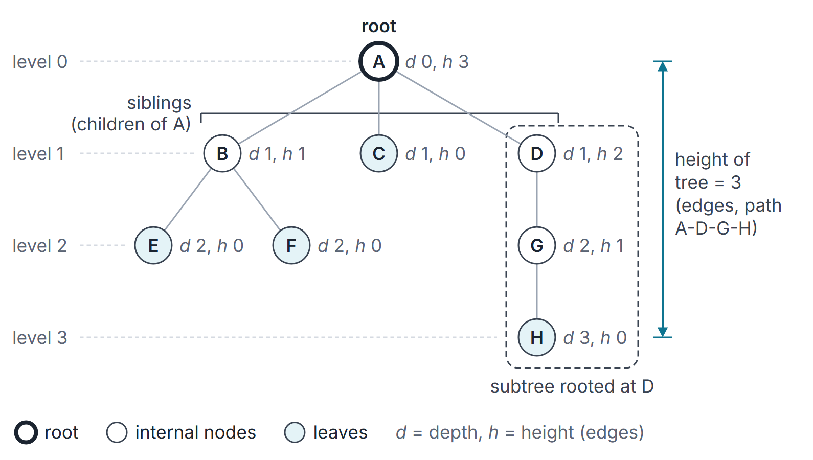
Tree terminology on one rooted tree — Figure 1. Root, internal nodes, leaves, depth and height marked on one rooted tree.

Height convention used in all Gate CS Mastery notes. Height counts edges. A single node has height 0 and the empty tree has height $-1$ . Some books count nodes instead, which adds 1 to every height. Before applying any formula in a question, check which convention the question uses; every height value shifts by 1, so height-dependent formulas need the matching convention; formulas unrelated to height do not change.

A non-empty tree with $n$ nodes has exactly $n-1$ edges, because every node except the root has exactly one edge to its parent.

Binary trees

A binary tree is either empty, or a root together with a left subtree and a right subtree, each of which is a binary tree. The left/right distinction matters: a root with only a left child and a root with only a right child are two different binary trees. This is what separates a binary tree from an ordered tree in which a node merely has "at most two" children.

Kinds of binary tree

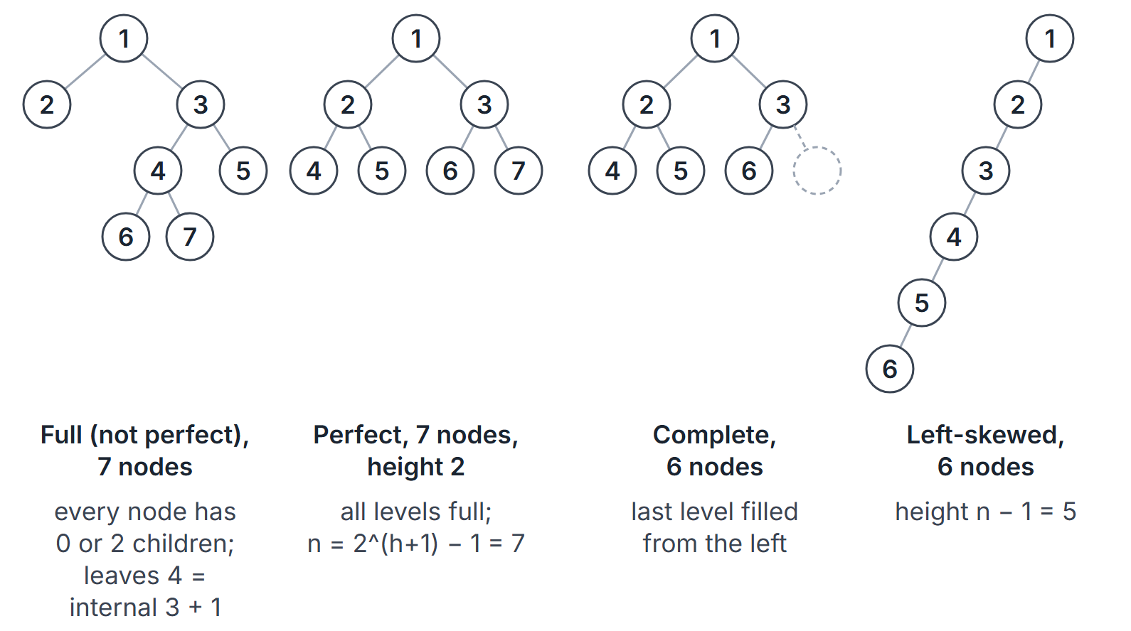
Names in this area differ between textbooks. The definitions below are the ones used throughout these notes; if a text uses a different meaning, check whether it defines the term.

Kind	Definition used here	Example property
Full (proper, strictly binary)	Every node has 0 or 2 children	$n = 2n_0 - 1$
Perfect	Full, and all leaves at the same depth	$n = 2^{h+1} - 1$
Complete	Every level full except possibly the last, which is filled from the left	height $= \lfloor \lg n \rfloor$
Skewed (degenerate)	Every internal node has exactly one child	height $= n - 1$
Balanced (informal)	Height is $O(\lg n)$ ; exact meaning depends on the scheme, for example AVL	see AVL Trees

Here $\lg$ means $\log_2$ . CLRS calls a perfect tree "complete" (Appendix B.5.3) and a heap-shaped tree "nearly complete" (Section 6.1); these notes use "complete" in the sense of the table.

Full, perfect, complete and skewed binary trees — Figure 2. The four kinds of binary tree side by side, each with 6 or 7 nodes.

Counting facts and their proofs

Let $n$ be the number of nodes, $h$ the height (edge convention), and $n_0, n_1, n_2$ the numbers of nodes with 0, 1 and 2 children.

Maximum and minimum number of nodes for a given height

Level $d$ of a binary tree holds at most $2^d$ nodes, since each node on level $d-1$ has at most two children. Summing over levels $0$ to $h$ :

n \le \sum_{d=0}^{h} 2^d = 2^{h+1} - 1 .

Equality holds exactly for the perfect tree. The minimum for height $h$ is $h + 1$ nodes (a skewed chain).

Turned around, a binary tree with $n$ nodes has height

\lceil \lg (n+1) \rceil - 1 \;\le\; h \;\le\; n - 1 ,

and $\lceil \lg(n+1) \rceil - 1 = \lfloor \lg n \rfloor$ for $n \ge 1$ . Example: with $n = 100$ , the minimum height is $\lfloor \lg 100 \rfloor = 6$ and the maximum is 99. The number of distinct binary trees with $n$ nodes and height $n-1$ is $2^{n-1}$ , since each of the $n - 1$ non-root nodes is independently a left or a right child.

Leaves versus two-child nodes: $n_0 = n_2 + 1$

Count edges two ways. Every node except the root has one parent edge, so there are $n - 1$ edges. Each node contributes as many edges as it has children, so there are $n_1 + 2n_2$ edges. With $n = n_0 + n_1 + n_2$ :

n_0 + n_1 + n_2 - 1 = n_1 + 2 n_2 \quad\Longrightarrow\quad n_0 = n_2 + 1 .

This holds for every non-empty binary tree, whatever its shape, and the number of one-child nodes $n_1$ does not appear. Two consequences:

A full binary tree has $n_1 = 0$ , so $n = 2n_0 - 1$ : it always has an odd number of nodes.
Worked example: a binary tree has 10 leaves and 5 nodes with one child. Then $n_2 = 9$ and $n = 10 + 5 + 9 = 24$ .

Null links: $n + 1$

For a nonempty tree ( $n\ge1$ ), in the linked representation each node has two child pointers, $2n$ pointers in total. Exactly $n - 1$ of them point to a node (one per edge), so

\text{null pointers} = 2n - (n-1) = n + 1 .

An empty tree has zero node child fields, edges and data-node leaves, and height $-1$ ; its separate root handle is null, not a child field. For the 24-node tree above there are 25 null links. Threaded binary trees reuse these $n+1$ null fields to store traversal links.

Extended-tree convention. Some texts (and discussions of "extended binary trees") replace each null link by a square external node. In that view there are exactly $n + 1$ external nodes, every original node is internal, and external nodes are the newly added leaves of the extended tree, not the original tree's data-node leaves. Check which meaning is in use.

Number of distinct binary trees: the Catalan numbers

Let $b_n$ be the number of structurally different binary trees with $n$ nodes (unlabelled shapes). Choosing a shape means choosing a left subtree with $k$ nodes and a right subtree with $n - 1 - k$ nodes:

b_0 = 1, \qquad b_n = \sum_{k=0}^{n-1} b_k\, b_{n-1-k} \quad (n \ge 1).

This is the Catalan recurrence, with closed form

b_n = C_n = \frac{1}{n+1}\binom{2n}{n}.

$n$	0	1	2	3	4	5	6	7
$C_n$	1	1	2	5	14	42	132	429

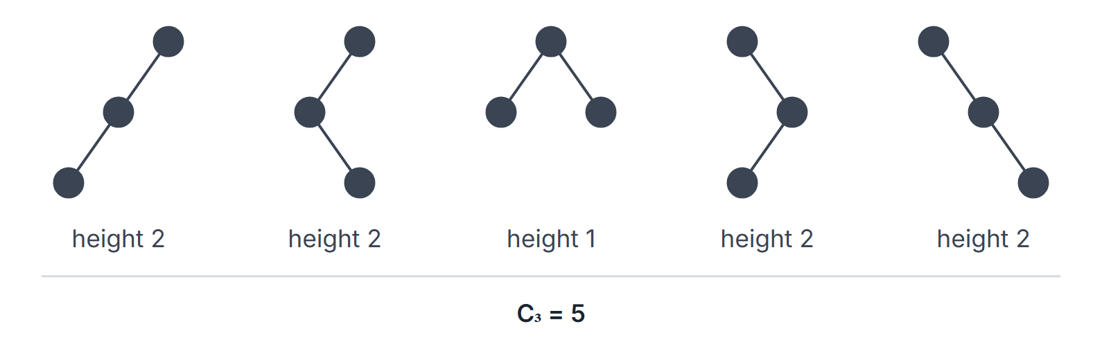
The five binary tree shapes with three nodes — Figure 3. All $C_3 = 5$ binary tree shapes with three nodes.

Read the question carefully for what is being counted:

Unlabelled shapes with $n$ nodes: $C_n$ .
Labelled binary trees with $n$ distinct labels placed anywhere: $n! \cdot C_n$ (for $n = 3$ : $6 \times 5 = 30$ ).
Binary search trees on $n$ distinct keys: $C_n$ , because the BST ordering fixes where each key goes once the shape is chosen (see Binary Search Trees).

Representing a binary tree

Linked representation

C

struct node {
    int key;
    struct node *left;   /* NULL if no left child  */
    struct node *right;  /* NULL if no right child */
};

Each node costs one key and two pointers; a parent pointer is added when upward moves are needed (for example, finding a successor without a stack). Space is $\Theta(n)$ for any shape.

Array (sequential) representation

Number the positions level by level, left to right, starting at 1 for the root. With 1-based indexing, for the node at index $i$ :

\text{left}(i) = 2i, \qquad \text{right}(i) = 2i + 1, \qquad \text{parent}(i) = \lfloor i/2 \rfloor \;(i > 1).

With 0-based indexing the formulas become $2i+1$ , $2i+2$ and $\lfloor (i-1)/2 \rfloor$ . Always state which base is in use.

The array form has no wasted slots for a complete binary tree, which is why binary heaps use it. For other shapes it wastes space: a right-skewed tree of height $h$ needs an array of size $2^{h+1} - 1$ to hold only $h + 1$ nodes.

For a complete binary tree with $n$ nodes stored this way, the leaves are exactly the indices $\lfloor n/2 \rfloor + 1, \ldots, n$ , so there are $\lceil n/2 \rceil$ leaves. Example: $n = 10$ gives leaves at indices 6 to 10, five leaves.

Which traversals determine a tree uniquely

A traversal lists the nodes in a fixed order: preorder (node, left, right), inorder (left, node, right), postorder (left, right, node) and level order (by depth, left to right). Assume all keys are distinct.

Given pair	Unique tree?	Why
Inorder + preorder	Yes	Preorder names the root; inorder splits the rest into left and right subtrees; recurse
Inorder + postorder	Yes	Same, with the root last in postorder
Inorder + level order	Yes	Level order names the root first; inorder splits; recurse on the subsequences
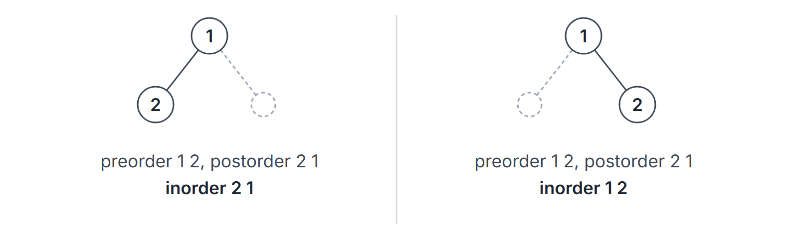
Preorder + postorder	Not in general	They cannot tell a lone left child from a lone right child. Exactly $2^{n_1}$ trees share one preorder and postorder pair, where $n_1$ is the number of one-child nodes, so the pair is unique exactly when $n_1 = 0$
Preorder + postorder, full binary tree	Yes	Every internal node has two children, so the split is forced
Level order + preorder, or level order + postorder	Not in general	Already fails for two nodes: root 1 with child 2 on either side gives the same level order, preorder and postorder
Any single traversal	No in general	For a BST with distinct keys, preorder alone, postorder alone or level order alone suffices, because inorder is the sorted order

The smallest counterexample: root 1 with left child 2, and root 1 with right child 2. Both have preorder 1, 2 and postorder 2, 1.

Two different trees with the same preorder and postorder — Figure 4. Preorder 1 2 and postorder 2 1 fit two different binary trees.

Worked example: rebuilding from preorder and inorder

Preorder: A B D E G C F H. Inorder: D B G E A C H F.

Preorder starts with A, so A is the root. In the inorder sequence, D B G E is left of A and C H F is right of A.
Left part: the next preorder symbols B D E G belong to it. B is its root; inorder D | B | G E puts D on the left and G E on the right.
Inside G E: preorder lists E before G, so E is the root, and inorder G E puts G as E's left child.
Right part: preorder C F H, inorder C H F. C is the root with nothing on its left; F H form its right subtree, with root F and H as F's left child.

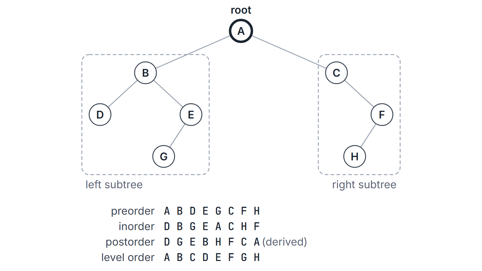
Tree rebuilt from preorder and inorder — Figure 5. The tree rebuilt from preorder A B D E G C F H and inorder D B G E A C H F.

Check: the rebuilt tree has postorder D G E B H F C A and level order A B C D E F G H.

Text

BUILD(pre[1..n], in[1..n])
    if n = 0 then return NIL
    r <- pre[1]
    k <- position of r in in[1..n]
    t <- new node with key r
    t.left  <- BUILD(pre[2..k], in[1..k-1])
    t.right <- BUILD(pre[k+1..n], in[k+1..n])
    return t

Searching for the root in the inorder array each time makes this $O(n^2)$ in the worst case (a skewed tree); using index-range/view arguments (no subarray copying) and a key-to-position map gives $\Theta(n)$ with $O(1)$ lookup (expected for hashing, or worst-case for suitable direct indexing). The map/output use $O(n)$ storage and recursion uses $O(h+1)$ stack. Naive linear lookup is $\Theta(n)$ best-case overall and $\Theta(n^2)$ worst-case; average-case analysis requires an input model and is deferred.

Important properties and observations

For a nonempty tree ( $n\ge1$ ): The edge count is always $n-1$ , whatever the shape.
For a nonempty tree ( $n\ge1$ ): $n_0 = n_2 + 1$ needs only "binary tree"; it does not need full or complete.
For a nonempty tree ( $n\ge1$ ): A full binary tree with $L$ leaves has $L - 1$ internal nodes and $2L - 1$ nodes.
For a nonempty tree ( $n\ge1$ ): A complete binary tree with $n$ nodes has height $\lfloor \lg n \rfloor$ and $\lceil n/2 \rceil$ leaves.
For a nonempty tree ( $n\ge1$ ): A perfect binary tree of height $h$ has $2^h$ leaves and $2^h - 1$ internal nodes.
Recursive algorithms on a tree of height $h$ use $O(h)$ stack space: $O(\lg n)$ on a balanced tree but $O(n)$ on a skewed one.

Common misconceptions.

"Complete" and "full" are different. A complete tree can have one node with a single (left) child; a full tree cannot.
"Number of binary trees with $n$ nodes" means shapes ( $C_n$ ) unless the question says the nodes are labelled.
Preorder plus postorder does not always fix a tree; inorder is needed unless the tree is full.

GATE examination perspective

Counting questions. Expect to use $n_0 = n_2 + 1$ , $2^{h+1} - 1$ , $n + 1$ null links and Catalan numbers. First identify the height convention and whether nodes are labelled.
Reconstruction questions. Given two traversals, rebuild the tree and report a third traversal or the height. Rebuild level by level and check by recomputing both given sequences.
Array index questions. Confirm whether the array is 0-based or 1-based before using parent and child formulas.
Trap: height off by one. If the answer choices differ by exactly 1, the convention is the point being tested.
Trap: assuming "binary tree" means "binary search tree". Ordering facts apply only to BSTs.

Summary

A binary tree is empty, or a root with an ordered pair of left and right binary subtrees.
Height in these notes counts edges: one node has height 0, the empty tree $-1$ .
For a nonempty tree ( $n\ge1$ ): At most $2^{h+1} - 1$ nodes for height $h$ ; height of an $n$ -node binary tree lies between $\lfloor \lg n \rfloor$ and $n-1$ .
For a nonempty tree ( $n\ge1$ ): $n_0 = n_2 + 1$ ; null links $= n + 1$ ; edges $= n - 1$ .
Shapes with $n$ nodes: $C_n = \frac{1}{n+1}\binom{2n}{n}$ (1, 1, 2, 5, 14, 42, ...).
Array form: children of $i$ at $2i$ and $2i+1$ (1-based); efficient only for complete trees.
With distinct keys, inorder plus any one of preorder, postorder or level order fixes a tree; preorder plus postorder fixes only full binary trees ( $2^{n_1}$ trees share a pair); level order plus preorder or postorder does not fix a tree. For a BST, any one of preorder, postorder or level order is enough.

Binary Tree Traversals: dependent. The traversal algorithms and their iterative versions.
Binary Search Trees: dependent. A binary tree with the search ordering.
Binary Heaps: dependent. A complete binary tree stored in an array.
AVL Trees: dependent. Keeping height $O(\lg n)$ .
Graph Theory Fundamentals: related. Trees as connected acyclic graphs.
Recurrence Relations: related. The Catalan recurrence.

Trees and Binary Trees

Introduction

Prerequisites