Binary Search Trees: short notes (Data Structures)

Introduction

A binary search tree (BST) is a binary tree that keeps its keys in order, so that searching can discard one whole subtree at every step. It supports the dynamic-set operations search, minimum, maximum, successor, predecessor, insert and delete, each in time proportional to the height of the tree.

BSTs solve a problem that sorted arrays solve only halfway: a sorted array gives $O(\lg n)$ search with binary search but needs $\Theta(n)$ time to insert or delete. A BST keeps search, insert and delete all at $O(h)$ , where $h$ is the height. The catch is that $h$ depends on the order in which keys arrive; this single fact drives the cost and shape analysis of BSTs.

BSTs are the basis of balanced trees such as AVL trees, of ordered maps in standard libraries, and of the multiway B-trees and B+ trees used for database indexes.

Prerequisites

Trees and Binary Trees: terminology, height convention (edges), Catalan numbers.
Binary Tree Traversals: inorder, preorder and postorder.
Recursion.

Core concepts

The BST property

Assume the keys are distinct unless stated otherwise. A binary tree is a BST if, for every node $x$ :

every key in the left subtree of $x$ is less than $x.key$ , and
every key in the right subtree of $x$ is greater than $x.key$ .

The condition is about whole subtrees, not just the two children. A tree where every node is larger than its left child and smaller than its right child can still violate the property deeper down. For example, root 50 with left child 30, and 30 with right child 60: each parent-child pair looks fine, but 60 sits in the left subtree of 50.

Duplicates. Textbooks differ. Common conventions are "equal keys go right", "equal keys go left", or "store a count in the node". A question with duplicate keys should state its rule; these notes use distinct keys.

Inorder traversal gives sorted order

By induction on the tree: inorder visits all of the left subtree (smaller keys, in sorted order by the inductive hypothesis), then the root, then all of the right subtree (larger keys, sorted). So inorder of a BST lists the keys in increasing order, in $\Theta(n)$ time. Consequences:

The inorder sequence of a BST is known as soon as the key set is known: it is the sorted key list.
Therefore a BST is fixed by its preorder alone (or its postorder alone, or its level order alone), because pairing that sequence with the sorted order rebuilds the tree.
The $k$ -th smallest key is the $k$ -th node visited by inorder.

Successor and predecessor

The successor of node $x$ is the node with the smallest key greater than $x.key$ .

If $x$ has a right subtree, the successor is the minimum of that subtree: go right once, then left as far as possible.
Otherwise, the successor is the lowest ancestor of $x$ whose left child is also an ancestor of $x$ (or $x$ itself). In words: go up until you arrive from a left child. If no such ancestor exists, $x$ holds the maximum and has no successor.

The predecessor is symmetric (maximum of the left subtree, or go up until you arrive from a right child). Both take $O(h)$ .

How the operations work

All pseudocode uses NIL for an empty pointer, <- for assignment, and nodes with fields key, left, right, p (parent).

Search

Text

BST-SEARCH(x, k)
    while x != NIL and k != x.key
        if k < x.key then x <- x.left
        else x <- x.right
    return x

The search follows one root-to-node path, so it examines at most $h + 1$ nodes.

Minimum and maximum

The minimum is the leftmost node: follow left pointers from the root until the next one is NIL. The maximum is the rightmost node. Neither needs a comparison of keys.

Insert

Text

BST-INSERT(T, z)          // z.left = z.right = NIL
    y <- NIL
    x <- T.root
    while x != NIL
        y <- x
        if z.key < x.key then x <- x.left
        else x <- x.right
    z.p <- y
    if y = NIL then T.root <- z          // tree was empty
    else if z.key < y.key then y.left <- z
    else y.right <- z

A new key always becomes a leaf. Existing nodes never move during insertion.

Delete: the three cases

Let $z$ be the node to delete.

$z$ is a leaf. Transplant it with NIL: if z.p = NIL, set T.root <- NIL; otherwise clear the appropriate child pointer of z.p.
$z$ has one child $c$ . If z.p = NIL, set T.root <- c; otherwise replace the appropriate child pointer of z.p by c. In either case set c.p <- z.p, including NIL when c becomes the root.
$z$ has two children. Find its successor $y$ , the minimum of $z$ 's right subtree. $y$ has no left child. Copy $y$ 's key into $z$ , then delete $y$ from the right subtree, which is case 1 or case 2. (Using the predecessor instead is equally valid; state which one is used. These notes use the successor.)

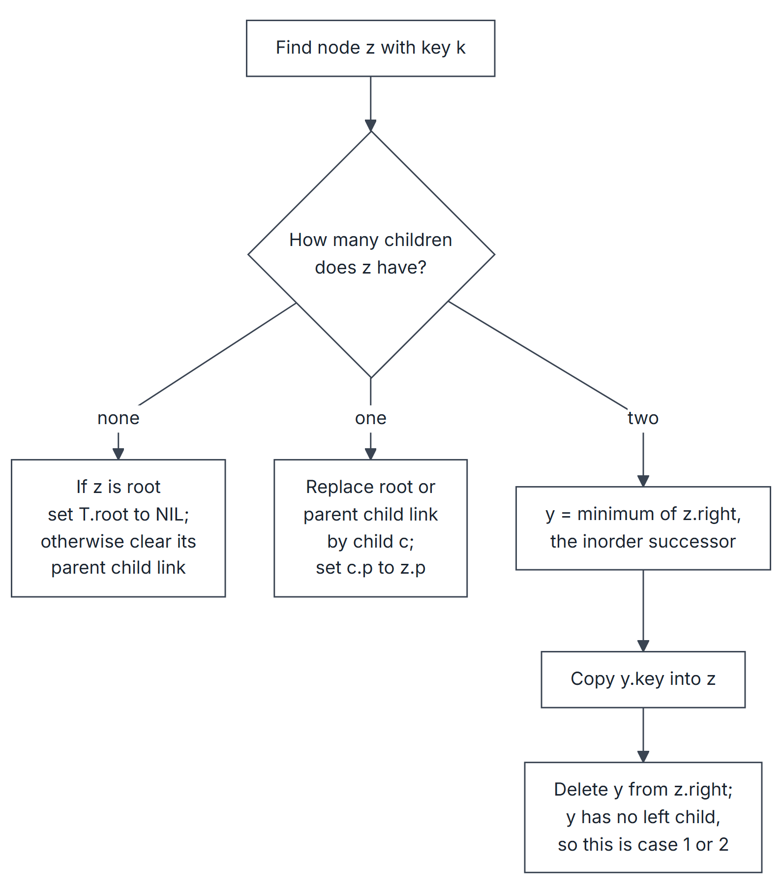
Decision flowchart for deleting a node z from a binary search tree by its number of children: none, one, or two, where the inorder successor's key is copied into z and the successor is then deleted. — Figure 1. Decision flow for BST deletion (successor version).

The "copy the key" form is the one used in the traces below. Library implementations often move the successor node itself instead of copying keys, so that pointers held elsewhere stay valid; the resulting tree shape is the same.

Worked example: build, search and delete

Insert, in this order, 50, 30, 70, 20, 40, 60, 80, 35, 45, 65 into an empty BST.

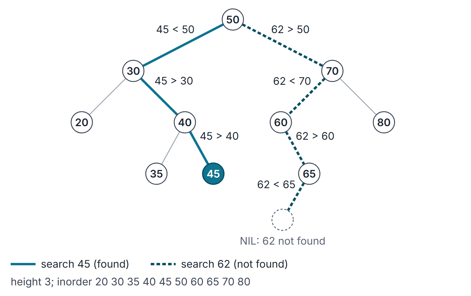
BST built from 50 30 70 20 40 60 80 35 45 65 with two search paths — Figure 2. The example BST, with the successful search path for 45 and the unsuccessful path for 62.

Root 50; left child 30 (children 20 and 40; 40 has children 35 and 45); right child 70 (children 60 and 80; 60 has right child 65).
Height: 3 (for example 50, 30, 40, 35).
Inorder: 20 30 35 40 45 50 60 65 70 80 (sorted, as expected).
Preorder: 50 30 20 40 35 45 70 60 65 80.
Postorder: 20 35 45 40 30 65 60 80 70 50.
Search 45 visits 50, 30, 40, 45: four nodes, so four comparisons to succeed.
Search 62 visits 50, 70, 60, 65 and then reaches NIL at 65's left: it fails after four comparisons. The last node where the search turned left (65) holds the smallest key greater than 62.
Counting convention. These counts use one (three-way) comparison per node visited. Code with separate != and < tests, such as BST-SEARCH above, makes up to two key comparisons per node: 7 for the search of 45 (two at each of 50, 30, 40 and one at 45) and 8 for the failed search of 62. Check which convention a question uses.

Now delete three keys in sequence, each from the tree left by the previous step.

Step	Case at that moment	Action	Preorder after the step	Inorder after the step
Delete 20	Leaf	30.left becomes NIL	50 30 40 35 45 70 60 65 80	30 35 40 45 50 60 65 70 80
Delete 60	One child (65)	65 replaces 60 as 70's left child	50 30 40 35 45 70 65 80	30 35 40 45 50 65 70 80
Delete 50 (root)	Two children	Successor = minimum of the right subtree = 65 (go to 70, then left to 65). Copy 65 into the root, then delete the old 65, a leaf	65 30 40 35 45 70 80	30 35 40 45 65 70 80

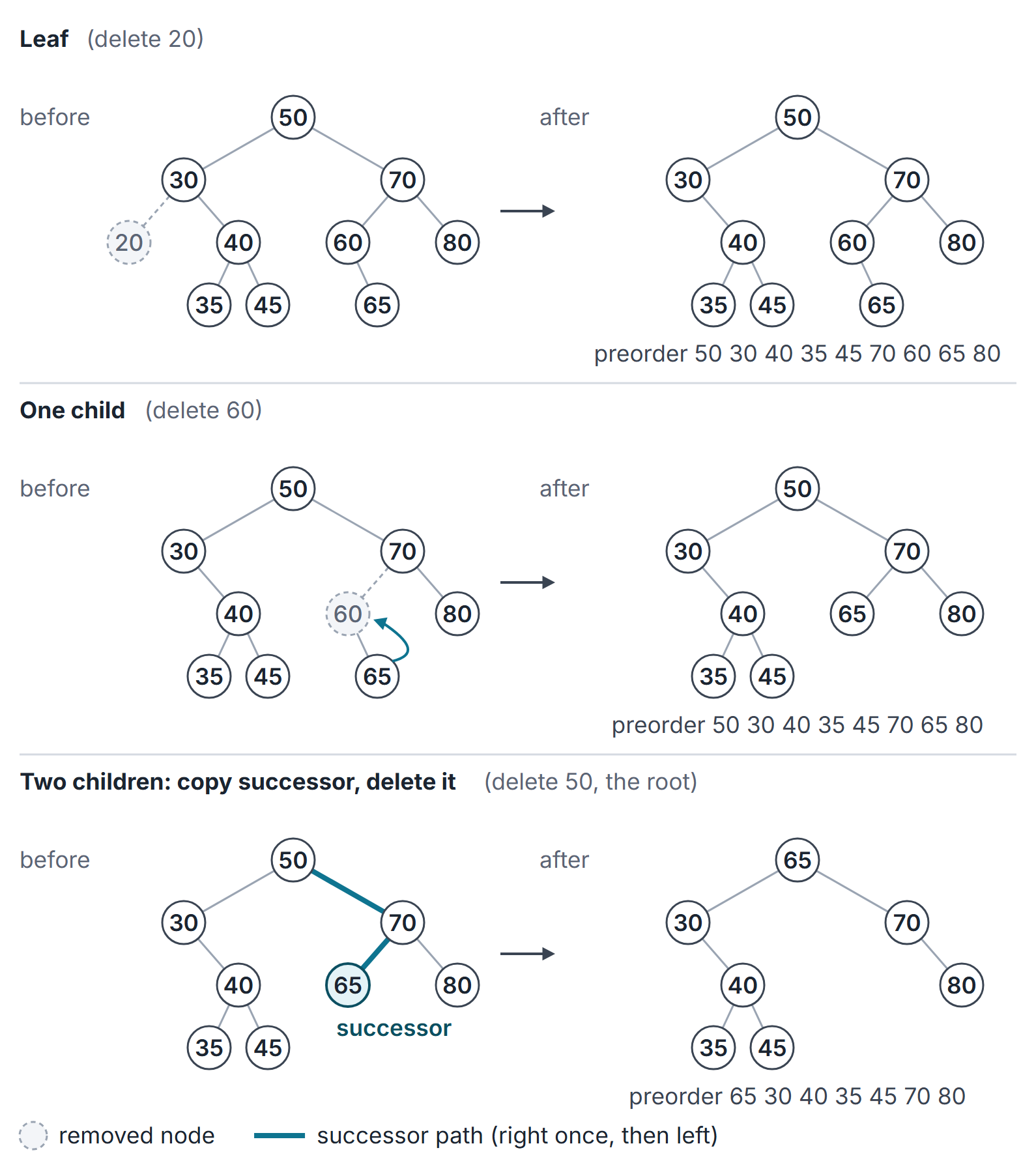
The three deletion cases on the example tree — Figure 3. Deletion of a leaf (20), a one-child node (60) and a two-child node (the root 50), each shown before and after.

Read the case from the tree at the moment of deletion. In the original tree, 30 has two children (20 and 40); deleting it there copies its successor 35 into it, giving preorder 50 35 20 40 45 70 60 65 80. But if 20 has already been deleted, 30 has only one child (40), and deleting 30 simply splices 40 into its place, giving preorder 50 40 35 45 70 60 65 80. Questions that delete several keys in order test exactly this.

Root edge cases. Deleting a singleton root sets T.root to NIL. Deleting a root with only a left or right child makes that child the new root and sets its parent to NIL. The same transplant rule handles a non-root leaf or one-child node; the two-child successor-copy convention is unchanged.

Height and running time

Every operation above walks one path from the root, so each runs in $O(h)$ time and $O(1)$ extra space (iterative versions), or $O(h)$ stack space (recursive versions).

Shape	Height $h$	Worst-case time of search, insert, delete for that shape
Balanced (complete) shape, $n\ge1$	$\lfloor \lg n \rfloor$	$\Theta(\lg n)$
Skewed shape (keys inserted in sorted or reverse-sorted order, or orders repeatedly choosing the smallest or largest remaining key)	$n - 1$	$\Theta(n)$
Average over random insertion orders (all $n!$ orders of distinct keys equally likely, insertions only)	expected $O(\lg n)$	expected $O(\lg n)$

The best case of any single search, on any shape, is $\Theta(1)$ : the key is at the root.

Points to note:

Inserting $1, 2, \ldots, n$ in increasing order produces a right-leaning chain. Searching for $n$ then compares against all $n$ keys. Building that tree costs $0 + 1 + \cdots + (n-1) = n(n-1)/2$ comparisons (one per node visited), which is $\Theta(n^2)$ .
Sorted order is not the only bad case. Of the $n!$ insertion orders of $n$ distinct keys, exactly $2^{n-1}$ give height $n - 1$ (for $n = 3, 4, 5$ : 4, 8 and 16 orders).
The expected-height result assumes random insertion order and no deletions. It says nothing about adversarial input; balanced trees such as AVL guarantee $O(\lg n)$ in the worst case.
Under a uniformly random permutation of distinct inserted keys, the expected height is $O(\lg n)$ ; no universal coefficient 2 is asserted here.

Counting BSTs

Given $n$ distinct keys, each shape of binary tree can be filled in exactly one way so that inorder is sorted. So the number of distinct BSTs on $n$ distinct keys equals the number of binary tree shapes, the Catalan number $C_n$ (1, 1, 2, 5, 14, 42, ...; closed form and table in Trees and Binary Trees). The BST view gives the recurrence directly: choose the root as the $k$ -th smallest key; the $k - 1$ smaller keys form the left BST and the $n - k$ larger keys form the right BST, so $b_n = \sum_{k=1}^{n} b_{k-1} b_{n-k}$ .

Different count: insertion orders producing one tree. The root must be inserted first; after that, the left and right subtree insertions may interleave in any way. For the perfect BST on 7 keys (root, two children, four leaves) the count is

\binom{6}{3} \times 2 \times 2 = 80

(choose which 3 of the remaining 6 positions go to the left subtree, times 2 valid orders inside each 3-node subtree).

Important properties and observations

Inorder of a BST is sorted; this is a complete test: a binary tree is a BST if and only if its inorder sequence is strictly increasing (distinct keys).
The minimum has no left child and the maximum has no right child. Neither is necessarily a leaf.
In the two-child delete case, the successor has no left child, which is why its own deletion is easy.
Given a BST's preorder, its postorder is determined. Example: preorder 40 25 10 30 28 35 60 50 70 65 gives inorder 10 25 28 30 35 40 50 60 65 70 and postorder 10 28 35 30 25 50 65 70 60 40 (height 3).
Checking the BST property by comparing each node only with its children is wrong; pass down a (low, high) range instead, or check that the inorder sequence increases.
Search, insert and delete are $O(h)$ , not $O(\lg n)$ . Write $O(\lg n)$ only when the tree is known to be balanced.

GATE examination perspective

Build and traverse. Insert a key sequence, then give a traversal, the height, or the number of nodes at some level. Draw the tree level by level and verify with inorder (must be sorted).
Preorder or postorder given. Rebuild the BST from one sequence using the ordering, then answer about the other traversals.
Delete sequences. Recheck each node's number of children at the moment of its deletion, and confirm whether the question uses the successor or the predecessor.
Counting. Number of BSTs on $n$ keys is $C_n$ ; number of insertion orders for a given shape uses the interleaving count.
Complexity traps. "Worst-case search in a BST" is $\Theta(n)$ ; "in a balanced BST" is $\Theta(\lg n)$ . Building a BST by $n$ insertions is $\Theta(n^2)$ worst case and expected $\Theta(n \lg n)$ for random orders.
Range questions. Keys that can appear on a search path form a nested interval sequence: after each comparison, later keys on the path must lie within the current (low, high) bounds. Use this to test whether a given sequence can be a search path.

Summary

Trees and Binary Trees: prerequisite. Shapes, height and Catalan counting.
Binary Tree Traversals: prerequisite. Inorder, preorder and postorder.
AVL Trees: dependent. Rotations that keep the height $O(\lg n)$ .
Searching: related. Binary search on arrays follows the same halving idea.
B-Trees and B+ Trees: related. Multiway search trees for disk-based indexes.
Binary Heaps: related. A different ordering (heap order) on a binary tree; compare what each supports efficiently.

Binary Search Trees

Introduction

Prerequisites