SQL Joins, Grouping, Aggregation and NULLs: short notes (Database Management Systems)

Revision mode

Introduction

Most real queries combine tables with joins, summarise rows with aggregate functions, and must cope with missing values. These three features interact: an outer join manufactures NULLs, aggregate functions skip NULLs, and the WHERE and HAVING filters drop anything whose condition is UNKNOWN. A query that looks like simple arithmetic often turns on one of these interactions.

The exact rules are fixed and then worked on one pair of tables so that every count can be traced row by row.

Prerequisites

SQL: Data Definition, Data Manipulation and Basic Queries: the SELECT block, bag semantics and the logical evaluation order.

Core concepts

Join syntax

Form	Meaning
`R JOIN S ON cond` (also `INNER JOIN`)	rows of $R \times S$ where `cond` is TRUE
`R NATURAL JOIN S`	equality on all columns with the same name; each such column appears once
`R JOIN S USING (c)`	equality on the listed common columns only
`R LEFT OUTER JOIN S ON cond`	inner join plus unmatched rows of $R$ padded with NULL
`R RIGHT OUTER JOIN S ON cond`	inner join plus unmatched rows of $S$
`R FULL OUTER JOIN S ON cond`	inner join plus unmatched rows of both

ON versus WHERE in an outer join. A condition in ON decides which pairs match; an unmatched left row still appears, padded. A condition in WHERE is applied after the join. A null-rejecting predicate such as salary > 55 removes padded rows because it is UNKNOWN for NULL, whereas salary IS NULL can retain them.

Aggregate functions

Function	NULL handling	On an empty input
`COUNT(*)`	counts rows, NULLs included	0
`COUNT(col)`	counts non-NULL values	0
`COUNT(DISTINCT col)`	counts distinct non-NULL values	0
`SUM(col)`, `AVG(col)`	ignore NULLs; mathematically, `AVG` = `SUM(col)` / `COUNT(col)` using real division (SQL integer division may differ)	NULL
`MIN(col)`, `MAX(col)`	ignore NULLs	NULL

Grouping

GROUP BY g partitions the rows that survive WHERE into groups with equal g; all NULLs of g form one group. Each group produces one output row. Under this note's strict grouping rule, every SELECT column must be grouped or aggregated. Functionally dependent selected columns are also permitted where the standard feature/dialect supports them. HAVING filters groups, after aggregation, and may use aggregates; WHERE filters rows, before grouping, and may not.

NULL and three-valued logic

Any arithmetic with NULL gives NULL, and any comparison with NULL (including NULL = NULL) gives UNKNOWN. Logical connectives follow the three-valued (Kleene) tables:

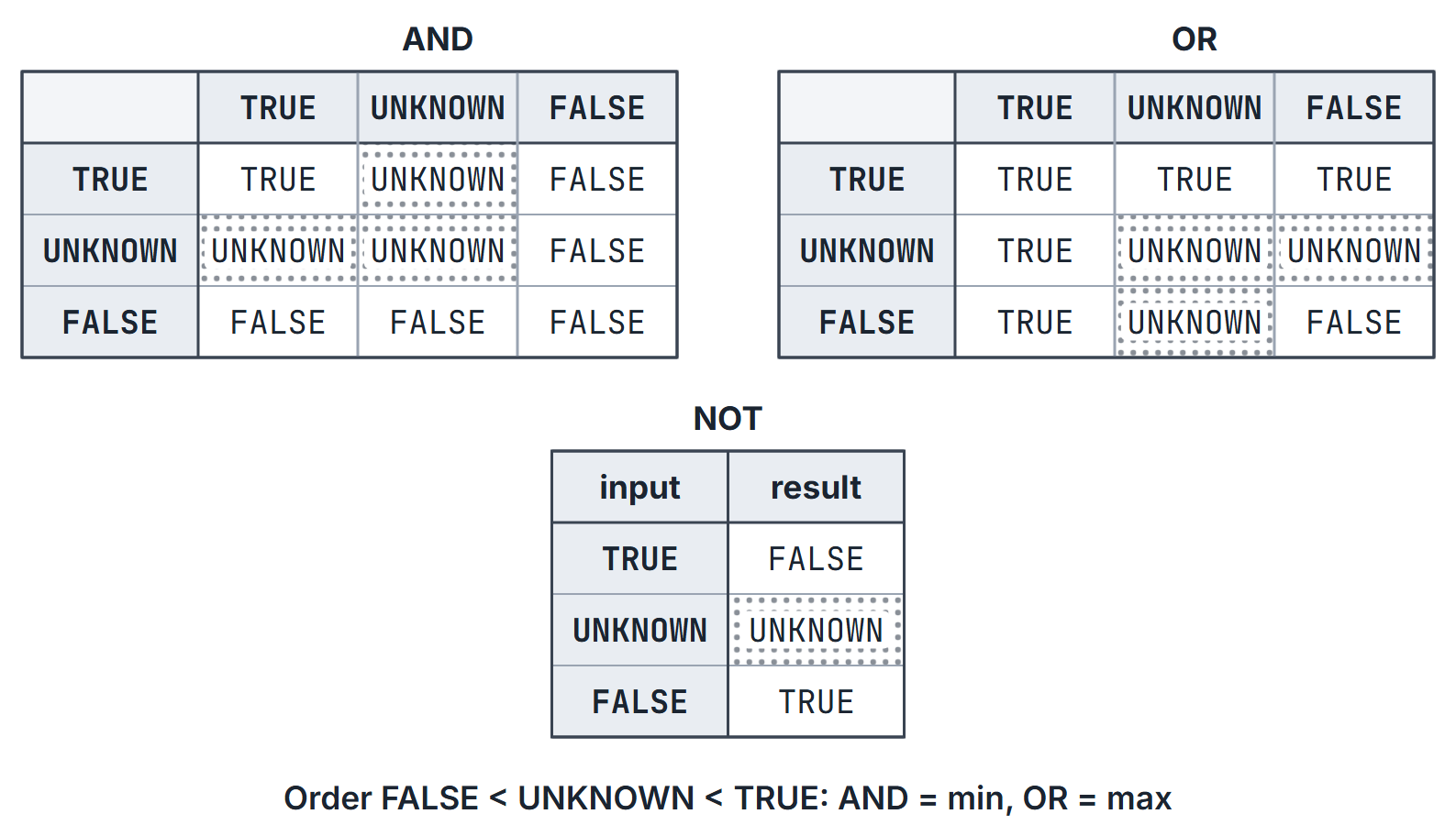
Truth tables of AND, OR and NOT over TRUE, UNKNOWN and FALSE — Figure 1. Three-valued logic: AND takes the minimum and OR the maximum under FALSE $<$ UNKNOWN $<$ TRUE; NOT swaps TRUE and FALSE and keeps UNKNOWN.

WHERE, HAVING and ON keep a row or group only when the condition is TRUE. CHECK constraints are the exception: a row passes a CHECK when the condition is TRUE or UNKNOWN.

How it works: the example tables

EMP(eid, name, dept, salary) and DEPT(dcode, dname):

eid	name	dept	salary
1	Asha	CS	70
2	Ravi	CS	50
3	Meena	EE	60
4	Kiran	EE	60
5	Arun	ME	40
6	Anil	NULL	55
7	Dev	CS	NULL

DEPT has rows (CS, Computer), (EE, Electrical), (ME, Mechanical), (CE, Civil). Department CE has no employee; Anil has no department; Dev has no salary.

Algorithms and pseudocode

Text

EVAL-GROUPED(block)
  T <- FROM with joins; keep rows whose WHERE condition is TRUE
  partition T by the GROUP BY columns (NULLs together)
  for each group G
      compute each aggregate over G, skipping NULL arguments (except COUNT(*))
      if HAVING is TRUE for G then output one row
  apply DISTINCT and ORDER BY

Grouping by sorting costs $O(n \lg n)$ for $n$ rows; hashing costs $O(n)$ expected.

Mathematical explanation

Why AVG is not SUM / COUNT(*). Interpreting the following quotients as real arithmetic (cast to a decimal/real SQL type when needed), with $n$ rows of which $k$ have a non-NULL value, AVG(col) $= \frac{1}{k}\sum \text{values}$ , while SUM(col) / COUNT(*) $= \frac{1}{n}\sum \text{values}$ . For $n\ge k>0$ , the denominators differ when $k<n$ , so the values can differ; they still agree if the sum is zero. For $k=0$ , AVG and SUM return NULL rather than the displayed numerical fractions.

Why COUNT(*) misleads after an outer join. A padded row is a real row: COUNT(*) counts it as 1 for a department with no employee. COUNT(e.eid) counts its NULL as nothing and gives the correct 0.

Three-valued logic as min and max. Order the values FALSE $<$ UNKNOWN $<$ TRUE. Then $a \wedge b = \min(a, b)$ , $a \vee b = \max(a, b)$ and $\neg$ reverses the order. Consequences: TRUE OR UNKNOWN is TRUE, FALSE AND UNKNOWN is FALSE, and p OR NOT p is UNKNOWN when $p$ is UNKNOWN.

Worked examples

Example 1: aggregates and NULL. Using real arithmetic for the displayed quotients (cast to decimal/real before SQL division), on EMP: COUNT(*) = 7, COUNT(salary) = 6, COUNT(dept) = 6, COUNT(DISTINCT dept) = 3, SUM(salary) = 335, AVG(salary) = $335 / 6 \approx 55.83$ , but SUM(salary) / COUNT(*) = $335 / 7 \approx 47.86$ .

Example 2: GROUP BY. SELECT dept, COUNT(*), COUNT(salary), AVG(salary) FROM EMP GROUP BY dept returns 4 groups:

dept	COUNT(*)	COUNT(salary)	AVG(salary)
NULL	1	1	55
CS	3	2	60
EE	2	2	60
ME	1	1	40

The CS average is $(70 + 50) / 2 = 60$ : Dev's NULL salary is skipped.

Example 3: HAVING versus WHERE.

... GROUP BY dept HAVING COUNT(*) >= 2 returns CS and EE.
... WHERE salary > 55 GROUP BY dept HAVING COUNT(*) >= 2 returns only EE: WHERE first keeps Asha, Meena and Kiran, leaving CS with one row.

Example 4: outer join and counting. SELECT d.dcode, COUNT(*), COUNT(e.eid) FROM DEPT d LEFT JOIN EMP e ON d.dcode = e.dept GROUP BY d.dcode gives CS 3 3, EE 2 2, ME 1 1, CE 1 0. The join itself has 7 rows: 6 matched (Anil matches nothing) plus the padded CE row.

Example 5: ON versus WHERE. DEPT d LEFT JOIN EMP e ON d.dcode = e.dept AND e.salary > 55 has 5 rows: (CS, Asha), (EE, Meena), (EE, Kiran), (ME, NULL), (CE, NULL). Moving e.salary > 55 to WHERE gives 3 rows, because the padded rows have salary NULL.

Example 6: aggregates on an empty set. SELECT COUNT(*), SUM(salary), MAX(salary) FROM EMP WHERE salary > 100 returns one row (0, NULL, NULL). With GROUP BY dept added, it returns no rows at all: there are no groups.

Example 7: NULL comparisons. SELECT COUNT(*) FROM EMP WHERE salary = NULL is 0; WHERE salary IS NULL is 1. WHERE salary > 55 OR salary <= 55 keeps 6 rows, not 7.

Example 8: NATURAL JOIN surprise. Suppose DEPT also had a column name holding the head of department's name, say Rao, Iyer, Das and Sen. EMP NATURAL JOIN DEPT equates every pair of same-named columns, which is only name; no employee is called Rao, Iyer, Das or Sen, so the result is empty. The intended match dept = dcode is never used, because those columns have different names. Prefer JOIN ... ON or USING.

SQLite differences. SQLite accepts a non-aggregated, non-grouped column in a grouped SELECT (for example SELECT dept, name FROM EMP GROUP BY dept) and returns a value from some row of the group; standard SQL rejects the query. RIGHT and FULL OUTER JOIN are supported only from SQLite 3.39.0. SQLite shows UNKNOWN as NULL.

Example 9: counting groups when NULLs are around. From the table of Example 2:

GROUP BY dept HAVING AVG(salary) > 55 returns CS and EE (both 60). Change the condition to >= 55 and the NULL-department group (Anil, 55) is returned too: a group whose key is NULL is still a group, and its HAVING test is evaluated like any other.
The query has 4 groups, while COUNT(DISTINCT dept) is 3: DISTINCT inside an aggregate skips the NULL, but GROUP BY makes a group for it.
HAVING COUNT(salary) = COUNT(*) keeps the groups with no NULL salary: the NULL-department group, EE and ME. CS fails because of Dev.

Important properties and observations

COUNT(*) counts rows, COUNT(col) counts non-NULL values.
Aggregates ignore NULLs; only COUNT returns 0 on empty input, the others NULL.
GROUP BY puts all NULLs in one group and DISTINCT treats them as equal, but = never matches two NULLs.
HAVING without GROUP BY treats the whole table as one group.
Outer join filters that reject NULL, such as salary > 55, belong in ON when padded rows must survive; WHERE with IS NULL may retain padded rows.
WHERE cannot contain aggregates; use HAVING or a subquery.
Inner join row count depends on matches only; an outer join adds exactly one row per unmatched row.

Common misconceptions.

"AVG(salary) treats NULL as 0." It skips NULL.
"NULL = NULL is TRUE." It is UNKNOWN; WHERE drops the row.
"p OR NOT p is always TRUE." Not when $p$ is UNKNOWN.

GATE examination perspective

Count the output rows. Consider a join plus GROUP BY plus HAVING query; process WHERE before grouping.
AVG with NULLs. Denominator is the number of non-NULL values.
COUNT(*) after LEFT JOIN. This gives 1, not 0, for an unmatched row.
Three-valued logic. Evaluate AND, OR, NOT with UNKNOWN; know that WHERE keeps only TRUE.
Empty input. COUNT gives 0, SUM and AVG give NULL; with GROUP BY, no row at all.

Summary

Sources

A. Silberschatz, H. F. Korth, S. Sudarshan, Database System Concepts, 7th ed., McGraw-Hill, 2019 (2020 copyright), 3.6 Null Values, 3.7 Aggregate Functions, 4.1 Join Expressions.
R. Elmasri, S. B. Navathe, Fundamentals of Database Systems, 7th ed., Pearson, 7.1 More Complex SQL Retrieval Queries.
SQLite documentation, consulted 2026-11-11: "The SELECT statement" (https://www.sqlite.org/lang_select.html) for bare columns in aggregate queries; release log of SQLite 3.39.0 (https://www.sqlite.org/releaselog/3_39_0.html) for RIGHT and FULL OUTER JOIN support.