SQL: Data Definition, Data Manipulation and Basic Queries: short notes (Database Management Systems)

Revision mode

Introduction

SQL is the standard language of relational databases. It has a data definition part (DDL) that creates and changes schemas and constraints, a data manipulation part (DML) that inserts, updates and deletes rows, and a query part built around the SELECT ... FROM ... WHERE block.

SQL is declarative like the calculus but is not the formal algebra: tables are multisets (bags), so duplicates survive unless DISTINCT removes them, and NULL brings a third truth value. To predict the output or the number of rows of a query on a small table, the exact semantics of each clause matters more than syntax.

Prerequisites

Relational Model and Keys: relations, primary and foreign keys, NULL.

Core concepts

Data definition

Text

CREATE TABLE EMP (
  eid    INT PRIMARY KEY,
  name   VARCHAR(20) NOT NULL,
  dept   CHAR(2),
  salary NUMERIC(8,2) CHECK (salary > 0),
  FOREIGN KEY (dept) REFERENCES DEPT(dcode)
);
ALTER TABLE EMP ADD phone VARCHAR(15);   -- new column, NULL in existing rows
DROP TABLE EMP;                          -- removes the schema and the data

Statement	Removes rows	Removes the table definition	Row-by-row WHERE
`DELETE FROM T WHERE p`	rows satisfying $p$ (all if no WHERE)	no	yes
`TRUNCATE TABLE T`	all rows	no	no
`DROP TABLE T`	all rows	yes	no

Data manipulation

INSERT INTO T VALUES (...) or INSERT INTO T SELECT ... (the query is evaluated fully before any row is inserted).
UPDATE T SET col = expr WHERE p: every condition and every subquery is evaluated on the table as it was before the statement; then all qualifying rows change.
DELETE FROM T WHERE p: the same rule; the condition is tested on the old table, then the rows are removed.

The basic query block

Text

SELECT [DISTINCT] A1, ..., Ak      -- projection (no duplicate removal without DISTINCT)
FROM   R1, ..., Rm                 -- Cartesian product of the listed tables
WHERE  P                           -- selection
ORDER BY A1 [ASC | DESC], ...      -- presentation order only

Its algebra meaning is $\pi_{A_1, \ldots, A_k}(\sigma_P(R_1 \times \cdots \times R_m))$ with bag semantics: the projection keeps one output row per input row unless DISTINCT is written.

Predicates.

Predicate	Meaning
`x BETWEEN a AND b`	$a \leq x \leq b$ , both ends included
`x IN (v1, v2)`	$x = v_1$ or $x = v_2$
`name LIKE 'A%'`	`%` matches any string (also empty), `_` exactly one character
`x IS NULL`, `x IS NOT NULL`	the only correct NULL tests; `x = NULL` is never true

How it works: the logical order of evaluation

A query is written SELECT first but evaluated in another order. Aliases defined in SELECT are therefore not visible in WHERE.

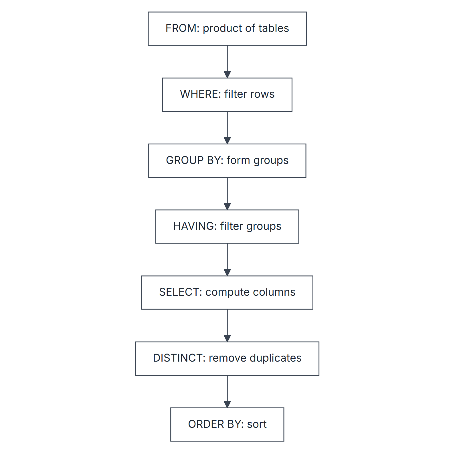
Flowchart of the logical evaluation order of a SELECT statement: FROM, WHERE, GROUP BY, HAVING, SELECT, DISTINCT, ORDER BY. — Figure 1. Logical evaluation order of the clauses of a SELECT statement; an optimiser may execute differently but must give the same result.

Grouping and HAVING are treated in SQL Joins, Grouping, Aggregation and NULLs.

Algorithms and pseudocode

The reference semantics of a single block, which any execution plan must match:

Text

EVAL-SELECT(block)
  T <- every combination of one row from each table in FROM   // bag, |T| = product of sizes
  T <- rows of T for which WHERE is TRUE                       // FALSE and UNKNOWN both dropped
  O <- for each row of T, the SELECT expressions                // one output row per row of T
  if DISTINCT then remove duplicate rows from O                 // NULLs count as equal here
  sort O by ORDER BY
  return O

Cost of the naive plan: $\prod_i |R_i|$ row combinations; real systems push the WHERE conditions into joins and use indexes.

Mathematical explanation

Bag semantics. Let a row $x$ occur $m$ times in the input. Selection keeps all $m$ copies or none; projection without DISTINCT keeps one output row per input row, so the count of an output row is the sum of the counts of the input rows that project to it. With DISTINCT, every count becomes 1. A FROM list of tables with $n_1, \ldots, n_m$ rows produces $n_1 n_2 \cdots n_m$ combinations before WHERE.

Three-valued WHERE. A comparison with NULL yields UNKNOWN, and WHERE keeps only rows whose condition is TRUE. So WHERE salary > 50 OR salary <= 50 drops rows whose salary is NULL, even though it looks like a tautology.

Worked examples

Table EMP(eid, name, dept, salary):

eid	name	dept	salary
1	Asha	CS	70
2	Ravi	CS	50
3	Meena	EE	60
4	Kiran	EE	60
5	Arun	ME	40
6	Anil	NULL	55

Example 1: duplicates. SELECT dept FROM EMP returns 6 rows. SELECT DISTINCT dept FROM EMP returns 4 rows: CS, EE, ME and one NULL. SELECT DISTINCT salary FROM EMP returns 5 rows (60 appears twice in the table).

Example 2: BETWEEN is inclusive. WHERE salary BETWEEN 50 AND 60 returns Ravi, Meena, Kiran and Anil: 4 rows.

Example 3: LIKE. WHERE name LIKE 'A%' returns Asha, Arun and Anil (3 rows). WHERE name LIKE '_r%' returns only Arun: the second character must be r.

Example 4: the NULL tautology. WHERE dept = 'CS' OR dept <> 'CS' returns 5 rows, not 6: Anil's dept is NULL, both comparisons are UNKNOWN, and the OR is UNKNOWN.

Example 5: UPDATE uses the old table. UPDATE EMP SET salary = salary + 10 WHERE salary < (SELECT AVG(salary) FROM EMP). The average of the old salaries is $335 / 6 \approx 55.83$ , so Ravi (50), Arun (40) and Anil (55) are raised: 3 rows change, to 60, 50 and 65. The subquery is not re-evaluated after each row changes.

Example 6: the size of a FROM list. With a second table DEPT of 3 rows, SELECT * FROM EMP, DEPT returns $6 \times 3 = 18$ rows; adding WHERE EMP.dept = DEPT.dcode keeps only matching pairs (Anil's NULL dept never matches).

Example 7: ORDER BY with ties. SELECT name FROM EMP ORDER BY salary DESC, name returns Asha, Kiran, Meena, Anil, Ravi, Arun: Kiran and Meena tie on 60 and are ordered by name.

SQLite differences from standard SQL (relevant when trying these on SQLite).

LIKE is case-insensitive for ASCII letters by default in SQLite; standard LIKE is case-sensitive.
7 / 2 is 3 in SQLite because both operands are integers; write 7.0 / 2 for 3.5.
SQLite sorts NULL before every other value in ascending order; the standard leaves the position of NULLs to the implementation unless NULLS FIRST or NULLS LAST is written.
SQLite has no TRUNCATE; DELETE FROM T without WHERE does the same job.
SQLite accepts a SELECT alias inside WHERE (SELECT salary * 2 AS d FROM EMP WHERE d > 100 runs); standard SQL rejects it because WHERE is evaluated before SELECT.

Important properties and observations

SELECT does not remove duplicates; DISTINCT does, and it treats all NULLs as one value.
FROM R, S is a Cartesian product; forgetting the join condition multiplies row counts.
WHERE keeps only TRUE; UNKNOWN rows vanish, which is how NULLs disappear from results.
Column aliases from SELECT cannot be used in WHERE (WHERE is evaluated first); most systems allow them in ORDER BY.
= NULL is never true; use IS NULL.
UPDATE and DELETE are set-at-a-time: conditions and subqueries see the old table.
ORDER BY is the only clause that guarantees order; without it, row order is unspecified.

Common misconceptions.

"SELECT A FROM R equals $\pi_A(R)$ ." Only with DISTINCT; without it, duplicates remain.
"BETWEEN 50 AND 60 excludes 60." It includes both ends.
"DELETE FROM T drops the table." It empties it; DROP TABLE removes the definition.

GATE examination perspective

Output size. Count rows with bag semantics: duplicates kept, DISTINCT collapses, products multiply.
NULL in WHERE. Rows with NULL in the compared column drop out of both = and <> filters.
Self-referencing UPDATE or DELETE. The condition is evaluated on the old table once.
SQL to algebra. Match a query with $\pi$ , $\sigma$ , $\times$ expressions, remembering duplicate handling.
DDL facts. DELETE versus TRUNCATE versus DROP; what ALTER TABLE ADD does to existing rows.

Summary

Sources

A. Silberschatz, H. F. Korth, S. Sudarshan, Database System Concepts, 7th ed., McGraw-Hill, 2019 (2020 copyright), 3.2 SQL Data Definition, 3.3 Basic Structure of SQL Queries, 3.4 Additional Basic Operations, 3.6 Null Values, 3.9 Modification of the Database.
R. Elmasri, S. B. Navathe, Fundamentals of Database Systems, 7th ed., Pearson, 6.1 SQL Data Definition and Data Types; 6.2 Specifying Constraints in SQL; 6.3 Basic Retrieval Queries in SQL; 6.4 INSERT, DELETE, and UPDATE Statements in SQL.
SQLite documentation, consulted 2026-11-11, for the SQLite differences listed in Worked examples, "SQL Language Expressions" (https://www.sqlite.org/lang_expr.html, LIKE case sensitivity), "The SELECT statement" (https://www.sqlite.org/lang_select.html, NULL position in ORDER BY), "DELETE" (https://www.sqlite.org/lang_delete.html, the truncate optimization).

Introduction

Prerequisites

Core concepts

Data definition

Data manipulation

The basic query block

How it works: the logical order of evaluation

Algorithms and pseudocode

Mathematical explanation

Worked examples

Important properties and observations

GATE examination perspective

Summary

Related topics

Sources

Next steps