Relational Algebra: short notes (Database Management Systems)

Introduction

Relational algebra is a procedural query language: a query is an expression built from operators that take relations and return a relation. Because the output of every operator is again a relation, operators compose freely, and an expression reads like a pipeline. Every SQL query is translated into an algebra expression before it is optimised and executed, so the algebra is also the vocabulary of query processing.

The algebra uses set semantics: relations have no duplicate tuples, and every operator removes duplicates from its result. This single fact explains several traps, such as the cardinality of a projection. What an expression returns on given tables, how many tuples a join can produce, and which expression expresses a "for all" query (division) are the standard calculations.

Prerequisites

Relational Model and Keys: relations as sets, keys and foreign keys.
Sets: union, intersection, difference and Cartesian product.

Core concepts

The six basic operators

Operator	Notation	Result
Selection	$\sigma_{p}(R)$	tuples of $R$ satisfying predicate $p$
Projection	$\pi_{A_1, \ldots, A_k}(R)$	the listed columns, duplicates removed
Union	$R \cup S$	tuples in either; $R$ , $S$ union-compatible
Set difference	$R - S$	tuples in $R$ and not in $S$ ; union-compatible
Cartesian product	$R \times S$	every pairing of a tuple of $R$ with a tuple of $S$
Rename	$\rho_{T(B_1, \ldots, B_n)}(R)$	same tuples, new relation and attribute names

Union compatibility. $R$ and $S$ have the same arity and corresponding attributes have the same domains. Names may differ; the result takes the names of $R$ .

These six are the fundamental operators: every derived operator can be written with them, and together they make a language relationally complete.

Derived operators

Operator	Definition with basic operators
Intersection $R \cap S$	$R - (R - S)$
Theta join $R \bowtie_{\theta} S$	$\sigma_{\theta}(R \times S)$
Equijoin	theta join whose $\theta$ is a conjunction of equalities
Natural join $R \bowtie S$	equality on all common attribute names, then one copy of each common attribute kept
Division $R \div S$ , $R(X, Y)$ , $S(Y)$	$\pi_X(R) - \pi_X\big((\pi_X(R) \times S) - R\big)$
Assignment $T \leftarrow E$	names an intermediate result

Outer joins

A natural or theta join drops a tuple that has no partner (a dangling tuple). Outer joins keep them, padding the missing attributes with NULL. The three outer joins are written as $R \mathbin{]\!\bowtie} S$ (left), $R \mathbin{\bowtie\![} S$ (right) and $R \mathbin{]\!\bowtie\![} S$ (full): the bracket marks the side whose dangling tuples are kept. Textbooks draw the same operators as a bowtie with extended horizontal strokes on the kept side.

Left outer join $R \mathbin{]\!\bowtie} S$ : all of $R \bowtie S$ plus each dangling tuple of $R$ padded with NULLs.
Right outer join $R \mathbin{\bowtie\![} S$ : plus each dangling tuple of $S$ .
Full outer join $R \mathbin{]\!\bowtie\![} S$ : plus dangling tuples of both.

In an ordinary equality/natural join, NULL equality is not TRUE, so NULL join keys do not match even each other. This does not apply to every theta predicate: IS NULL, null-safe equality or a TRUE OR branch can permit a match; evaluate the specified predicate.

How it works: the joins on one pair of tables

Take $R(A, B) = \{(1, a), (2, b), (3, a), (4, c)\}$ and $S(B, C) = \{(a, x), (a, y), (b, x), (d, z)\}$ .

Tables R(A, B) and S(B, C) and the results of their natural join (5 tuples), left outer join (6 tuples, adding 4, c, NULL), right outer join (6 tuples, adding NULL, d, z) and full outer join (7 tuples) — Figure 1. Natural, left outer, right outer and full outer join of the same two tables; dangling tuples are padded with NULL.

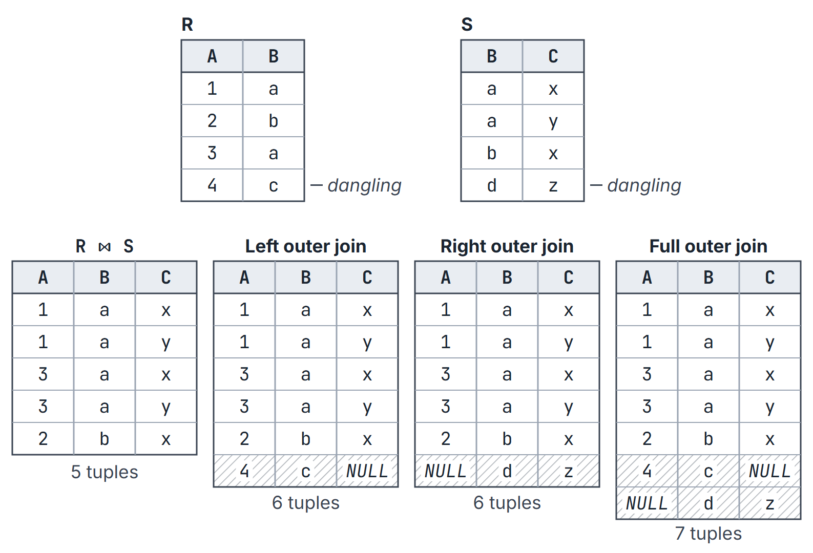
$R \times S$ has $4 \times 4 = 16$ tuples and attributes $A, R.B, S.B, C$ .
$R \bowtie S$ matches on $B$ : $(1, a, x), (1, a, y), (3, a, x), (3, a, y), (2, b, x)$ : 5 tuples.
$R \mathbin{]\!\bowtie} S$ adds $(4, c, \text{NULL})$ : 6 tuples. $R \mathbin{\bowtie\![} S$ adds $(\text{NULL}, d, z)$ : 6 tuples. $R \mathbin{]\!\bowtie\![} S$ : 7 tuples.
$\pi_B(R) = \{a, b, c\}$ : 3 tuples, not 4, because the two $a$ values merge.

Algorithms and pseudocode

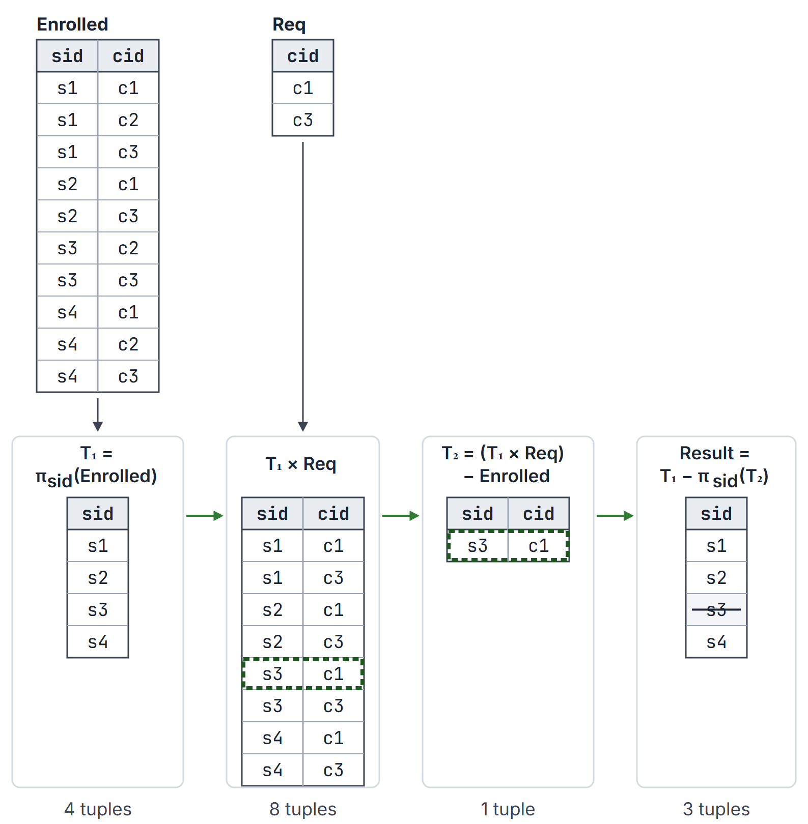
Division answers "which $x$ are related to every $y$ in $S$ ". The textbook expression works in three steps:

Text

DIVIDE(R(X, Y), S(Y))
  T1 <- pi_X(R)                  // every candidate x
  T2 <- (T1 x S) - R             // pairs (x, y) that WOULD be needed but are missing
  T3 <- pi_X(T2)                 // x values missing at least one y
  return T1 - T3

A direct evaluation sorts or hashes $R$ by $X$ and counts, for each $x$ , how many distinct $y$ of $S$ it has; $x$ qualifies when the count equals $|S|$ . After hashing $S$ for expected $O(1)$ membership tests, sorting $R$ gives expected $O(|S|+|R|\lg|R|)$ time; sorting both inputs requires accounting for both sorting costs.

Nested-loop evaluation of $R \bowtie_\theta S$ costs $|R| \cdot |S|$ predicate tests; hash join on an equality costs $O(|R| + |S| + \text{output})$ on average.

Mathematical explanation

Cardinality bounds for $|R| = m$ , $|S| = n$ , both non-empty:

Expression	Minimum	Maximum
$\sigma_p(R)$	0	$m$
$\pi_L(R)$	1	$m$
$R \cup S$	$\max(m, n)$	$m + n$
$R \cap S$	0	$\min(m, n)$
$R - S$	$\max(0, m - n)$	$m$
$R \times S$	$m n$	$m n$
$R \bowtie S$	0	$m n$
$R \bowtie_\theta S$	0	$m n$
$R \bowtie S$ , common attributes a key of $S$	0	$m$
$R \mathbin{]\!\bowtie} S$	$m$	$m n$
$R \mathbin{\bowtie\![} S$	$n$	$m n$
$R \mathbin{]\!\bowtie\![} S$	$\max(m, n)$	$\max(m n, m + n)$
$R(X, Y) \div S(Y)$	0	$\lfloor m / n \rfloor$

Join with a foreign key. If the common attributes of $R$ and $S$ form a foreign key of $R$ , declared NOT NULL and referencing the primary key of $S$ , then every tuple of $R$ matches exactly one tuple of $S$ and $|R \bowtie S| = |R|$ .

Where the outer-join bounds come from. Write $j = |R \bowtie S|$ , $d_R$ and $d_S$ for the numbers of dangling tuples. Then $|R \mathbin{]\!\bowtie\![} S| = j + d_R + d_S$ .

Maximum: either everything matches everything ( $j = m n$ , nothing dangles) or nothing matches ( $j = 0$ , all $m + n$ tuples dangle). The larger wins, so for $m = n = 1$ the maximum is 2, not 1.
Minimum: every tuple of either side appears in at least one output tuple, so the result has at least $\max(m, n)$ tuples; this is reached when each tuple of the smaller side matches exactly one tuple of the larger and the rest of the larger side dangles. For two 4-tuple relations, as in Figure 1, the full outer join has between 4 and 16 tuples; Figure 1 has 7.
If the common attributes are a key of $S$ , each $R$ tuple matches at most one $S$ tuple, so the inner join has at most $m$ tuples; the minimum 0 needs only that no value matches.

Natural join special cases. With no common attributes, $R \bowtie S = R \times S$ . With identical schemas, $R \bowtie S = R \cap S$ . Always $R \bowtie R = R$ .

Why the division formula is right. $x$ is in the result iff $(x, y) \in R$ for every $y \in S$ . $\pi_X(R) \times S$ lists every pair that would be required; subtracting $R$ leaves exactly the required-but-missing pairs; their $x$ values are the ones that fail, and removing them from the candidates leaves the answer. If $S$ is empty, nothing is required, nothing fails, and $R \div S = \pi_X(R)$ .

Worked examples

Example 1: division. Enrolled(sid, cid) = $\{(s_1, c_1), (s_1, c_2), (s_1, c_3), (s_2, c_1), (s_2, c_3), (s_3, c_2), (s_3, c_3), (s_4, c_1), (s_4, c_2), (s_4, c_3)\}$ .

Divided by Req(cid) = $\{c_1, c_3\}$ : $\{s_1, s_2, s_4\}$ . Here $T_2 = \{(s_3, c_1)\}$ , so $T_3 = \{s_3\}$ .
Divided by $\{c_1, c_2, c_3\}$ : $\{s_1, s_4\}$ .
Divided by the empty relation: $\{s_1, s_2, s_3, s_4\}$ .

The relation Enrolled with 10 tuples divided by Req containing c1 and c3: the intermediate pi_sid(Enrolled) x Req minus Enrolled leaves s3 with c1, so the result is s1, s2 and s4 — Figure 2. Division step by step: the only required pair missing from Enrolled is $(s_3, c_1)$ , so the result is $\{s_1, s_2, s_4\}$ .

Example 2: maximum without aggregation. For $R(A) = \{3, 7, 5\}$ , the largest value is

\pi_A(R) - \pi_{R.A}\big(\sigma_{R.A < T.A}(R \times \rho_T(R))\big)

The subtracted part is every value smaller than some other value, $\{3, 5\}$ , so the result is $\{7\}$ .

Example 3: "at least two courses". $\pi_{E_1.sid}\big(\sigma_{E_1.sid = E_2.sid \wedge E_1.cid \neq E_2.cid}(\rho_{E_1}(\text{Enrolled}) \times \rho_{E_2}(\text{Enrolled}))\big)$ on the Enrolled relation of Example 1 returns all four students; "exactly one course" would be $\pi_{sid}(\text{Enrolled})$ minus that result, which is empty here.

Example 4: projection then selection order. $\pi_A(\sigma_{B = a}(R)) = \{1, 3\}$ on the $R$ of Figure 1, but $\sigma_{B = a}(\pi_A(R))$ is not even well formed: $B$ was projected away. Selection and projection commute only when the projection keeps every attribute that the predicate uses.

Example 5: join with a foreign key. EMP(eno, dno) with 5 rows and dno a NOT NULL foreign key to DEPT(dno, dname) with 3 rows: $|EMP \bowtie DEPT| = 5$ whatever the data. If 2 employees had dno NULL instead, the natural join would have 3 tuples and the left outer join 5.

Important properties and observations

Set semantics. Projection and union remove duplicates; $|\pi_L(R)|$ can be less than $|R|$ unless $L$ contains a key.
Selections cascade and commute: $\sigma_{p \wedge q}(R) = \sigma_p(\sigma_q(R)) = \sigma_q(\sigma_p(R))$ .
Projections cascade: $\pi_{L_1}(\pi_{L_2}(R)) = \pi_{L_1}(R)$ when $L_1 \subseteq L_2$ .
Selection distributes over $\cup$ , $\cap$ and $-$ ; projection distributes over $\cup$ but not over $\cap$ or $-$ . Example: $R = \{(1, a)\}$ , $S = \{(1, b)\}$ : $\pi_1(R \cap S) = \emptyset$ but $\pi_1(R) \cap \pi_1(S) = \{1\}$ .
Natural inner joins are commutative and associative (up to attribute order); theta joins require correctly reassociated predicates, and outer joins are excluded; $\times$ and $\bowtie$ are the expensive operators, so optimisers push selections below them.
Difference is not commutative; $R - S$ and $S - R$ differ in general.
Mixing inner and outer joins is not associative: $(R \mathbin{]\!\bowtie} S) \bowtie T$ can differ from $R \mathbin{]\!\bowtie} (S \bowtie T)$ . A selection on an attribute of the padded side also cannot be pushed below an outer join: $\sigma_{C = x}(R \mathbin{]\!\bowtie} S)$ on Figure 1 has 3 tuples, $R \mathbin{]\!\bowtie} \sigma_{C = x}(S)$ has 4.

Related material. Aggregation and grouping $_{G}\gamma_{F}(R)$ , duplicate elimination and sorting belong to the extended algebra used for SQL; the GATE syllabus algebra is the set-based core above. Semi-join $R \ltimes S = \pi_{R}(R \bowtie S)$ appears in distributed query processing.

Common misconceptions.

" $|R \bowtie S| \leq \max(|R|, |S|)$ ." No: up to $|R| \cdot |S|$ , when every tuple matches every tuple.
" $R \div S$ is empty when $S$ is empty." No: it is $\pi_X(R)$ .
"Natural join compares NULLs as equal." It does not; NULL never satisfies an equality.

GATE examination perspective

Evaluate an expression. Work on small tables: track duplicates removed by projection and NULL padding of outer joins.
Cardinality questions. Minimum and maximum tuples of a join, union or difference; joins on a foreign key.
"For all" queries. These are division; recognise the $\pi - \pi((\pi \times S) - R)$ shape even when written without $\div$ .
Equivalence of expressions. Which rewrites (pushing selection, distributing projection) are valid.
Self-joins with rename. Apply this to "at least two", "maximum" and "pairs" queries.

Summary

Basic, independent operators: $\sigma$ , $\pi$ , $\cup$ , $-$ , $\times$ , $\rho$ ; the classical derived operators intersection, inner joins and division derive from them. NULL-padding outer joins and aggregation are extensions.
Set semantics: every result is duplicate-free; projection can shrink the tuple count.
Natural join equates all common attributes; no common attributes gives the Cartesian product.
Outer joins keep dangling tuples with NULL padding; NULL does not match in ordinary equality/natural joins; arbitrary predicates must be evaluated.
Division $R \div S = \pi_X(R) - \pi_X((\pi_X(R) \times S) - R)$ answers "related to all"; dividing by an empty relation returns $\pi_X(R)$ .
$|R \bowtie S|$ ranges from 0 to $|R| \cdot |S|$ ; a NOT NULL foreign key to a key makes it exactly $|R|$ .
Selection distributes over $\cup$ , $\cap$ , $-$ ; projection only over $\cup$ .
Maximum, "at least two" and similar queries use self-joins with rename and difference.

Relational Model and Keys: prerequisite; relations as sets and keys.
Sets: prerequisite; the set operations underneath.
SQL: Data Definition, Data Manipulation and Basic Queries: related; SQL queries map to algebra expressions, with bag semantics.
Tuple Relational Calculus: dependent; the declarative language with the same expressive power for safe queries.

Relational Algebra

Introduction

Prerequisites

Core concepts

The six basic operators

Derived operators

Outer joins

How it works: the joins on one pair of tables

Algorithms and pseudocode

Mathematical explanation

Worked examples

Important properties and observations

GATE examination perspective

Summary

Sources

Next steps

Introduction

Prerequisites

Core concepts

The six basic operators

Derived operators

Outer joins

How it works: the joins on one pair of tables

Algorithms and pseudocode

Mathematical explanation

Worked examples

Important properties and observations

GATE examination perspective

Summary

Related topics

Sources

Next steps