Basic Blocks and Control-Flow Graphs: short notes (Compiler Design)

Revision mode

Introduction

Optimisation and code generation work on three-address code organised into basic blocks: maximal straight-line sequences that control enters only at the top and leaves only at the bottom. Inside a block every instruction runs if the first one does, so local transformations (common subexpressions, dead code, register use) can reason about it as a unit. Between blocks, the control-flow graph (CFG) records which block can follow which, and global analyses such as reaching definitions and liveness run over it.

Loops matter most, since programs spend most of their time in them. Dominators, back edges and natural loops identify loops in a CFG without reference to the source syntax. The core tasks are finding the leaders of a code fragment and counting blocks and edges; dominators and natural loops are covered later as related material.

Prerequisites

Intermediate Representations: Syntax Trees, DAGs and Three-Address Code: three-address instructions, conditional and unconditional jumps.
Directed graphs, reachability and depth-first search (see the note Translating Expressions and Control Flow for how jumps are generated).

Core concepts

Leader. The first instruction of a basic block. The rules: (1) the first instruction of the program is a leader; (2) any instruction that is the target of a jump is a leader; (3) any instruction immediately after a conditional or unconditional jump is a leader. Return and other terminators count as unconditional transfers to procedure exit; if code follows, it begins a new block.
Basic block. A leader and all instructions after it up to, but not including, the next leader (or the end).
Flow graph. Nodes are basic blocks. There is an edge $B \to C$ if $C$ 's first instruction can run right after $B$ 's last: either $B$ ends in a jump to $C$ 's leader, or $C$ follows $B$ in program order and $B$ does not end in an unconditional jump (or return). An entry node points to the first block and the blocks that leave the program point to an exit node.
Dominator. $d$ dominates $n$ ( $d \operatorname{dom} n$ ) if every path from the entry to $n$ goes through $d$ . Every node dominates itself. The immediate dominator of $n \ne$ entry is its closest strict dominator; the immediate-dominator relation forms the dominator tree.
Back edge. An edge $a \to h$ whose head dominates its tail: $h \operatorname{dom} a$ .
Natural loop of a back edge $a \to h$ . The header $h$ plus all nodes that can reach $a$ without passing through $h$ . The header dominates every node of the loop and is its only entry.
Reducible flow graph. Every retreating edge (one that goes against a depth-first ordering) is a back edge. Structured code (if, while, for, break, continue) always gives reducible graphs.

How it works

Example 1: partitioning into blocks

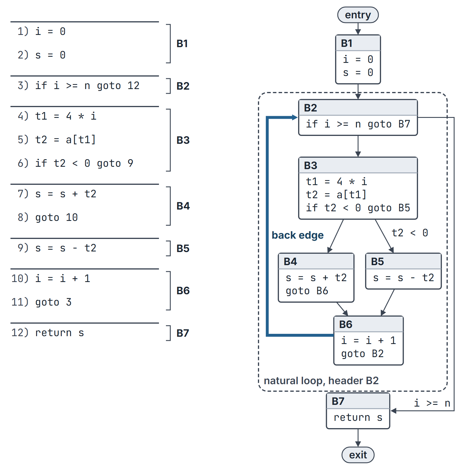
The program below sums the absolute values of the $n$ elements of an integer array a (4 bytes per element):

Text

 1) i = 0
 2) s = 0
 3) if i >= n goto 12
 4) t1 = 4 * i
 5) t2 = a[t1]
 6) if t2 < 0 goto 9
 7) s = s + t2
 8) goto 10
 9) s = s - t2
10) i = i + 1
11) goto 3
12) return s

Applying the leader rules:

Instruction	Why it is a leader
1	First instruction
3	Target of the jump in 11
4	Follows the conditional jump 3
7	Follows the conditional jump 6
9	Target of the jump in 6
10	Target of the jump in 8
12	Target of the jump in 3; follows the jump 11

Instruction 9 also follows the jump 8. The seven leaders give seven blocks: $B_1 = \{1, 2\}$ , $B_2 = \{3\}$ , $B_3 = \{4, 5, 6\}$ , $B_4 = \{7, 8\}$ , $B_5 = \{9\}$ , $B_6 = \{10, 11\}$ , $B_7 = \{12\}$ .

The flow graph has 8 edges between blocks:

From	To	Reason
$B_1$	$B_2$	Falls through
$B_2$	$B_7$	Jump taken ( $i \ge n$ )
$B_2$	$B_3$	Falls through
$B_3$	$B_5$	Jump taken ( $t_2 < 0$ )
$B_3$	$B_4$	Falls through
$B_4$	$B_6$	Unconditional jump; no fall-through to $B_5$
$B_5$	$B_6$	Falls through
$B_6$	$B_2$	Unconditional jump

With the entry and exit nodes there are also the edges entry $\to B_1$ and $B_7 \to$ exit.

Leaders, basic blocks and flow graph of the absolute-sum loop — Figure 1. The 12 instructions split at leaders 1, 3, 4, 7, 9, 10 and 12 into blocks B1 to B7, and the flow graph with 8 edges between blocks; the edge B6 to B2 is a back edge and its natural loop is B2 to B6.

Example 2: nested loops and a self-loop

Text

 1) i = 1
 2) if i > n goto 10
 3) j = 1
 4) t = i * j
 5) s = s + t
 6) j = j + 1
 7) if j <= n goto 4
 8) i = i + 1
 9) goto 2
10) if s > 100 goto 12
11) s = 100
12) return s

Leaders: 1 (first); 2 (target of 9); 3 (after the jump 2); 4 (target of 7, a backward jump); 8 (after the jump 7); 10 (target of 2, and after the jump 9); 11 (after the jump 10); 12 (target of 10). Eight blocks: $B_1 = \{1\}$ , $B_2 = \{2\}$ , $B_3 = \{3\}$ , $B_4 = \{4, \ldots, 7\}$ , $B_5 = \{8, 9\}$ , $B_6 = \{10\}$ , $B_7 = \{11\}$ , $B_8 = \{12\}$ .

The 10 edges are $B_1 \to B_2$ ; $B_2 \to B_3$ and $B_2 \to B_6$ ; $B_3 \to B_4$ ; $B_4 \to B_4$ and $B_4 \to B_5$ ; $B_5 \to B_2$ ; $B_6 \to B_7$ and $B_6 \to B_8$ ; $B_7 \to B_8$ . The jump in 7 goes back to the first instruction of its own block, so $B_4$ has an edge to itself. A one-instruction block such as $B_2$ is normal: a conditional jump that is also a jump target forms a block alone.

Related material. Dominators, back edges and natural loops, in this section and the next, go beyond the GATE syllabus. Its optimisation items are local optimisation and three data-flow analyses: those need basic blocks and flow graphs, but not loop detection. Dominators and natural loops are kept because they define which cycles count as loops for loop optimisations.

Dominators

The dominator sets satisfy

D(\text{entry}) = \{\text{entry}\}, \qquad D(n) = \{n\} \cup \bigcap_{p \in pred(n)} D(p)

and are computed iteratively, starting every non-entry $D(n)$ at the set of all nodes and repeating until nothing changes. This is a forward data-flow problem whose meet is intersection.

For the example (taking $B_1$ as the first node):

Node	Dominators	Immediate dominator
$B_1$	$B_1$	none
$B_2$	$B_1, B_2$	$B_1$
$B_3$	$B_1, B_2, B_3$	$B_2$
$B_4$	$B_1, B_2, B_3, B_4$	$B_3$
$B_5$	$B_1, B_2, B_3, B_5$	$B_3$
$B_6$	$B_1, B_2, B_3, B_6$	$B_3$
$B_7$	$B_1, B_2, B_7$	$B_2$

$B_6$ is not dominated by $B_4$ or $B_5$ , since each of them can be bypassed by the other branch. A direct check: $d$ dominates $n$ exactly when deleting $d$ makes $n$ unreachable from the entry.

Back edges and natural loops

Of the 8 edges, only $B_6 \to B_2$ has a head that dominates its tail, so it is the one back edge. Its natural loop is found by searching backward from the tail $B_6$ without passing the header $B_2$ : $B_6$ , then $B_4$ and $B_5$ , then $B_3$ , and $B_2$ itself. The loop is $\{B_2, B_3, B_4, B_5, B_6\}$ with header $B_2$ . $B_1$ and $B_7$ are outside it.

Loops with the same header. If two back edges have the same header, their natural loops are usually merged and treated as one loop. If two natural loops have different headers, they are either disjoint or one is nested inside the other.

Example 2, dominators and loops. The dominator sets are $D(B_1) = \{B_1\}$ , $D(B_2) = \{B_1, B_2\}$ , $D(B_3) = \{B_1, B_2, B_3\}$ , $D(B_4) = \{B_1, \ldots, B_4\}$ , $D(B_5) = \{B_1, \ldots, B_5\}$ , $D(B_6) = \{B_1, B_2, B_6\}$ , $D(B_7) = \{B_1, B_2, B_6, B_7\}$ and $D(B_8) = \{B_1, B_2, B_6, B_8\}$ . Two edges are back edges:

$B_4 \to B_4$ : every node dominates itself, so a self-loop is always a back edge. Its natural loop is $\{B_4\}$ , the inner loop over j.
$B_5 \to B_2$ : the backward search from $B_5$ finds $B_4$ , then $B_3$ (and $B_4$ again through its self-loop), stopping at the header $B_2$ . The loop is $\{B_2, B_3, B_4, B_5\}$ , the outer loop over i, and it contains the inner loop.

$B_7 \to B_8$ and $B_6 \to B_8$ go forward, so $B_8$ has two predecessors and is not in any loop.

An irreducible graph. With entry $E$ and edges $E \to A$ , $E \to B$ , $A \to B$ , $B \to A$ , the cycle $A \leftrightarrow B$ has two entries. Neither $A$ nor $B$ dominates the other, so neither cycle edge is a back edge and the cycle is not a natural loop. Such graphs arise only from unrestricted goto.

Next-use within a block

Related material. For register allocation inside a block, the code generator scans the block backward and records for each name whether it is live and where its next use is. At the end of a block, temporaries are usually dead and user variables are assumed live unless global analysis says otherwise. Global liveness, the general form of this idea, is treated in the note Liveness Analysis.

Blocks and the hardware

A block ends at every branch, and a branch is exactly where a pipelined processor risks a control hazard; scheduling instructions within a block and laying out blocks so that the common path falls through both reduce the cost of these hazards (see Pipeline Hazards).

Important properties and observations

Every instruction belongs to exactly one block, and the blocks partition the program in order.
The number of blocks equals the number of leaders.
An unconditional jump has one successor edge; a conditional jump has two (taken and fall-through), unless both coincide.
A block with a single exit never falls through after goto or return, so the next block in program order is not automatically a successor.
Dominance is reflexive, antisymmetric and transitive, and the strict dominators of a node form a chain ordered by the dominator tree.
Loop entry is unique: in a natural loop only the header has predecessors outside the loop.

Common misconceptions.

"The instruction after a jump is a leader only for conditional jumps." It is a leader after any jump.
"A jump instruction starts a block." A jump ends its block; its target and its successor start blocks.
"Every cycle in a CFG is a natural loop." Only cycles entered through a dominating header, as in the irreducible example.

GATE examination perspective

Find leaders and count blocks. Apply this to a numbered three-address fragment; remember all three rules, including targets of backward jumps.
Self-loops and one-instruction blocks. A backward jump to its own block's leader gives an edge from a block to itself (Example 2, $B_4$ ); count it as one edge.
Count flow-graph edges. One per jump target plus one per fall-through from a block not ending in goto or return.
Dominators and immediate dominators. Use a drawn CFG; the dominator tree.
Back edges and natural loops. Check $h \operatorname{dom} a$ , then search backward from the tail.
Loop-invariant code and induction variables. These are moved or simplified only within natural loops, which is why loop detection comes first.

Summary

Leaders: first instruction, jump targets, and instructions after jumps. A block runs from a leader to before the next.
Flow-graph edges: jump targets and fall-throughs (not after goto or return).
Example: leaders 1, 3, 4, 7, 9, 10, 12; seven blocks; 8 edges between blocks.
$d \operatorname{dom} n$ if every entry-to- $n$ path passes $d$ ; computed by $D(n) = \{n\} \cup \bigcap D(pred)$ .
Back edge $a \to h$ with $h \operatorname{dom} a$ ; its natural loop is $h$ plus nodes reaching $a$ without $h$ .
Example: back edge $B_6 \to B_2$ , loop $\{B_2, \ldots, B_6\}$ .
Example 2: leaders 1, 2, 3, 4, 8, 10, 11, 12; eight blocks; 10 edges including the self-loop $B_4 \to B_4$ ; loops $\{B_4\}$ inside $\{B_2, B_3, B_4, B_5\}$ .

Sources

A. V. Aho, M. S. Lam, R. Sethi, J. D. Ullman, Compilers, Principles, Techniques, and Tools, 2nd ed., Pearson Addison-Wesley, 2007: Section 8.4 (basic blocks, next-use information, flow graphs, representation of flow graphs, loops), Section 9.6 (dominators, depth-first ordering, back edges and reducibility, natural loops).