Constant Propagation: short notes (Compiler Design)

Introduction

If a variable holds the same known constant on every path to a use, the compiler can replace the use by the constant. That enables constant folding (computing 4 * 2 at compile time), which can make more variables constant, and can make branch conditions known so that whole paths become dead. Constant propagation is the global analysis that finds these facts.

Unlike reaching definitions or liveness, its data-flow values are not sets of facts but a small lattice per variable: "not yet known", "this constant", or "not a constant". It is the textbook example of a framework that is monotone but not distributive, so the iterative solution can be less precise than the meet over all paths. Questions ask for the value of a variable at a point, the meet rules, or why the analysis loses precision at joins.

Prerequisites

Data-Flow Analysis Framework: semilattices, meet, transfer functions, the iterative algorithm, MOP and MFP.
Three-address code and basic blocks (see the note Basic Blocks and Control-Flow Graphs).

Core concepts

Values for one variable. UNDEF (no constant information yet: optimistic top; it can propagate through assignments whose operands are UNDEF), a constant $c$ , or NAC (not a constant: different values on different paths, or a value unknown at compile time, such as input).
Order. UNDEF is the top element, the constants form one level with no order among them, NAC is the bottom. $x \le y$ means $x$ is less precise.
Meet for one variable.

\text{UNDEF} \wedge v = v, \qquad \text{NAC} \wedge v = \text{NAC}, \qquad c \wedge c = c, \qquad c_1 \wedge c_2 = \text{NAC}\ (c_1 \ne c_2)

Data-flow value of a point. A map $m$ from every variable to one of these values; the meet of two maps is taken variable by variable.
Direction and boundary. Forward; at the entry every variable is UNDEF; every other block also starts at UNDEF for every variable (the top).

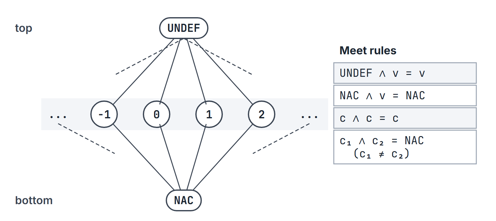
Figure 1. The constant-propagation semilattice for one variable: UNDEF at the top, every constant such as -1, 0, 1, 2 on one middle level with no order among them, and NAC at the bottom; two different constants meet in NAC, and UNDEF meet c is c.

How it works

Transfer functions

For an instruction $s$ and input map $m$ , the output map $m'$ equals $m$ except for the variable assigned by $s$ :

Statement	New value of $x$
$x = c$ (a constant)	$c$
$x = y \mathbin{op} z$	if $m(y)$ and $m(z)$ are constants, $m(y) \mathbin{op} m(z)$ ; else if either is NAC, NAC; else UNDEF
$x = y$	$m(y)$
$x$ = input, a call result, or a load through a pointer	NAC

A block's transfer function is the composition of its instructions'. The iterative algorithm is the forward one: $IN[B]$ is the meet of the predecessors' $OUT$ maps, $OUT[B] = f_B(IN[B])$ , repeated until nothing changes.

Example 1: a loop

Text

B1: i = 1
    k = 4
B2: j = k * 2          (loop body; B2 -> B2 and B2 -> B3)
    i = i + 1
B3: m = j + k

First pass: $IN[B_2] = OUT[B_1] = \{i{:}1, k{:}4\}$ ; $B_2$ gives $j = 8$ , $i = 2$ .
Second pass: $IN[B_2] = OUT[B_1] \wedge OUT[B_2]$ , and for $i$ , $1 \wedge 2 = \text{NAC}$ ; $k$ stays 4 and $j$ stays 8.
Final: at the exit of $B_3$ , $i$ = NAC, $j = 8$ , $k = 4$ , $m = 12$ .

So j = k * 2 can become j = 8, m = j + k can become m = 12, and only i must stay a variable. Iteration stops because each value can fall at most twice (UNDEF to a constant to NAC).

The passes in the order $B_1, B_2, B_3$ , written for $B_2$ :

Pass	$IN[B_2]$	$OUT[B_2]$
1	$i{:}1,\ k{:}4$ ( $OUT[B_2]$ is still all UNDEF)	$i{:}2,\ j{:}8,\ k{:}4$
2	$i{:}\text{NAC},\ j{:}8,\ k{:}4$	$i{:}\text{NAC},\ j{:}8,\ k{:}4$
3	no change	no change

In pass 2, $j$ at the start of $B_2$ is $\text{UNDEF} \wedge 8 = 8$ : on the path from $B_1$ , $j$ has not been assigned yet, and the optimistic meet ignores that path. The third pass only confirms the fixed point.

Example 2: a variable defined on only one path

Text

B1: c = input; if c goto B2 else B3
B2: x = 5
B3: w = 1
B4: y = x + 1          (B2 -> B4, B3 -> B4)

At $B_4$ , $x$ is $5 \wedge \text{UNDEF} = 5$ , so $y = 6$ . The rule UNDEF $\wedge\, v = v$ is optimistic: it assumes the path on which $x$ was never assigned does not lead to a meaningful use of $x$ . A program that reads an uninitialised variable has no defined value there, so the compiler may pick any.

Example 3: nondistributivity

Text

B1: c = input; if c goto B2 else B3
B2: x = 3
    y = 2
B3: x = 2
    y = 3
B4: z = x + y          (B2 -> B4, B3 -> B4)

On each path, $z = 5$ : the meet over all paths (MOP) gives $z = 5$ . The iterative algorithm meets first: at $IN[B_4]$ , $x = 3 \wedge 2 = \text{NAC}$ and $y = 2 \wedge 3 = \text{NAC}$ , so $z = \text{NAC}$ . The maximum fixed point (MFP) is NAC.

The cause is that the transfer function $f$ of $B_4$ does not distribute over meet:

f(m_1 \wedge m_2) = f(\{x{:}\text{NAC}, y{:}\text{NAC}\}) \Rightarrow z = \text{NAC}, \qquad f(m_1) \wedge f(m_2) \Rightarrow z = 5 \wedge 5 = 5

The framework is still monotone: if $m \le m'$ then $f(m) \le f(m')$ , so the iteration converges, and the result is safe ( $\text{MFP} \le \text{MOP}$ ). It is just not as precise as the ideal.

Example 4: propagation, folding and dead-code elimination in one block

Text

a = 3
b = a + 2
c = a * b
d = c - 10
e = d * x          (x is read from input, so it is NAC)
f = b * 4

Propagating and folding instruction by instruction gives $a = 3$ , $b = 5$ , $c = 15$ , $d = 5$ , then $e = 5 * x$ (still NAC, since $x$ is NAC) and $f = 20$ . The block becomes a = 3, b = 5, c = 15, d = 5, e = 5 * x, f = 20. If only $e$ and $f$ are live on exit, the first four assignments are now dead and dead-code elimination removes them:

Text

e = 5 * x
f = 20

Six instructions become two. Constant propagation itself deletes nothing; it rewrites uses, and the deletions come from the liveness-based clean-up that follows (see the note Liveness Analysis).

Transfer-function details that decide answers

An operand that is UNDEF and one that is NAC give NAC; an UNDEF operand with a constant gives UNDEF. The table above lists the cases in exactly that priority: both constant, then any NAC, then UNDEF.
Algebraic identities are a separate rule. With $y$ NAC, x = y * 0 gives $x$ = NAC under the transfer function above, although $x$ is always 0 at run time. A compiler that also applies the identity $y \times 0 = 0$ (for integers) finds the constant; the basic framework does not.
A copy passes the value through: after x = y with $y = 7$ , $x = 7$ , so a chain of copies of a constant stays constant.
A variable reassigned to the same constant on every path stays constant, even inside a loop: if both $B_1$ and a loop body assign t = 3, every meet is $3 \wedge 3 = 3$ .

Constant propagation and dead branches

When a condition becomes a constant, one successor is unreachable. The basic algorithm still includes the unreachable path in the meet, which can make values NAC needlessly:

Text

B1: k = 1
    if k == 1 goto B2 else B3
B2: y = 2              (B2 -> B4)
B3: y = 3              (B3 -> B4)
B4: z = y + 1

Control always reaches $B_4$ through $B_2$ , so $z$ is always 3. The basic analysis meets $y = 2$ from $B_2$ with $y = 3$ from $B_3$ and reports $y$ and $z$ as NAC at $B_4$ .

Related material. A conditional variant propagates values only along edges already known to be executable: it starts with the entry alone, and at a branch whose condition is a known constant it marks only the selected edge. On the program above it never marks $B_1 \to B_3$ , so $B_3$ contributes nothing to the meet and the analysis finds $y = 2$ and $z = 3$ . This variant is not part of the basic framework summarised here.

Constant propagation and SSA

In SSA form each variable has exactly one definition, so the constant value of a name can be propagated directly from its definition to all uses, and $\phi$ -functions perform the meet at joins: $x_3 = \phi(x_1, x_2)$ with $x_1 = 3$ , $x_2 = 3$ gives $x_3 = 3$ ; with $x_2 = 2$ it gives NAC.

Important properties and observations

Height of the lattice per variable is 3 levels (UNDEF, constants, NAC), so each variable changes at most twice and the iteration terminates quickly.
The constant level is infinite but flat: no two constants are comparable, so the lattice still has finite height.
Monotone, not distributive: MFP can be strictly below MOP (Example 3).
Meet with UNDEF is optimistic; meet with NAC is pessimistic. Mixing up the two is the most common error.
Folding and propagation feed each other: a folded constant can make further expressions constant, which is why the analysis is iterated rather than done in one pass.
Pointer stores and calls make every variable they might change NAC unless alias information proves otherwise.
Values at the entry stay UNDEF for every variable: UNDEF is the top/no-information-yet lattice value in the order used here, distinct from NAC (known not to be a single constant). It can propagate through assignments with UNDEF operands, so it does not prove that the destination has no definition. Analysis initialization is not itself a diagnosis of source-language uninitialized use.

Common misconceptions.

"If a variable is constant on every path, the analysis will find it." Not if the constant comes from different values combined after the join (Example 3).
"UNDEF means not a constant." UNDEF is the top (no information yet); NAC is the bottom.
"Constant propagation is backward." It is forward: values flow from definitions to later uses.
"Constant propagation removes the dead assignments." It only replaces uses by constants; dead-code elimination removes assignments whose targets are no longer live (Example 4).
"x = y * 0 always makes $x$ a constant." Only if the algebraic identity is applied; the standard transfer function gives NAC when $y$ is NAC.

GATE examination perspective

Value of a variable at a point. After constant propagation: apply the meet rules at joins and fold constants inside blocks.
Meet table. UNDEF with $c$ , $c$ with $c$ , $c_1$ with $c_2$ , anything with NAC.
Nondistributivity. Recognise the $x = 3, y = 2$ versus $x = 2, y = 3$ pattern and state that the iterative result is NAC while each path gives a constant.
Properties. Forward, monotone, not distributive, finite height; MFP $\le$ MOP.
Effect on code. Which instructions can be replaced by constants and which branches become decidable.
Clean-up counts. After propagation, folding and dead-code elimination with given live-out variables, how many instructions remain (Example 4: six become two).
Iteration traces. The value of a variable in $IN[B]$ after a given pass; the first pass ignores the back edge (Example 1, pass table).

Summary

Data-Flow Analysis Framework: prerequisite. The iterative algorithm, semilattices, and MOP versus MFP.

Constant Propagation

Introduction

Prerequisites

Core concepts

How it works

Transfer functions

Example 1: a loop

Example 2: a variable defined on only one path

Example 3: nondistributivity

Example 4: propagation, folding and dead-code elimination in one block

Transfer-function details that decide answers

Constant propagation and dead branches

Constant propagation and SSA

Important properties and observations

GATE examination perspective

Summary

Sources

Next steps

Introduction

Prerequisites

Core concepts

How it works

Transfer functions

Example 1: a loop

Example 2: a variable defined on only one path

Example 3: nondistributivity

Example 4: propagation, folding and dead-code elimination in one block

Transfer-function details that decide answers

Constant propagation and dead branches

Constant propagation and SSA

Important properties and observations

GATE examination perspective

Summary

Related topics

Sources

Next steps